Difference between revisions of "Evolution of Universe"
| (15 intermediate revisions by 2 users not shown) | |||
| Line 6: | Line 6: | ||
=== Problem 1 === | === Problem 1 === | ||
Rewrite the first Friedman equation in terms of redshift and analyze the contributions of separate components at different stages of Universe evolution. | Rewrite the first Friedman equation in terms of redshift and analyze the contributions of separate components at different stages of Universe evolution. | ||
| − | <div class="NavFrame collapsed"> | + | <!--<div class="NavFrame collapsed"> |
<div class="NavHead">solution</div> | <div class="NavHead">solution</div> | ||
<div style="width:100%;" class="NavContent"> | <div style="width:100%;" class="NavContent"> | ||
| Line 13: | Line 13: | ||
</p> | </p> | ||
</div> | </div> | ||
| − | </div></div> | + | </div>--></div> |
<div id="SCM11"></div> | <div id="SCM11"></div> | ||
<div style="border: 1px solid #AAA; padding:5px;"> | <div style="border: 1px solid #AAA; padding:5px;"> | ||
| + | |||
=== Problem 2 === | === Problem 2 === | ||
Find the time dependence for the scale factor and analyze asymptotes of the dependence. Plot $a(t)$. | Find the time dependence for the scale factor and analyze asymptotes of the dependence. Plot $a(t)$. | ||
| − | <div class="NavFrame collapsed"> | + | <!--<div class="NavFrame collapsed"> |
<div class="NavHead">solution</div> | <div class="NavHead">solution</div> | ||
<div style="width:100%;" class="NavContent"> | <div style="width:100%;" class="NavContent"> | ||
| − | <p style="text-align: left;"> | + | <p style="text-align: left;"></p> |
| − | + | ||
| − | + | ||
</div> | </div> | ||
| − | </div></div> | + | </div>--></div> |
| − | + | ||
| Line 34: | Line 32: | ||
<div id="SCM12"></div> | <div id="SCM12"></div> | ||
<div style="border: 1px solid #AAA; padding:5px;"> | <div style="border: 1px solid #AAA; padding:5px;"> | ||
| + | |||
=== Problem 3 === | === Problem 3 === | ||
Determine the redshift value corresponding to equality of radiation and matter densities. | Determine the redshift value corresponding to equality of radiation and matter densities. | ||
| Line 52: | Line 51: | ||
</div> | </div> | ||
</div></div> | </div></div> | ||
| − | |||
| − | |||
| Line 60: | Line 57: | ||
<div style="border: 1px solid #AAA; padding:5px;"> | <div style="border: 1px solid #AAA; padding:5px;"> | ||
=== Problem 4 === | === Problem 4 === | ||
| − | Construct effective one-dimensional potential (see [[Solutions_of_Friedman_equations_in_the_Big_Bang_model#dyn15|problem]] | + | Construct effective one-dimensional potential (see [[Solutions_of_Friedman_equations_in_the_Big_Bang_model#dyn15|problem]] of Chapter 3) |
<div class="NavFrame collapsed"> | <div class="NavFrame collapsed"> | ||
<div class="NavHead">solution</div> | <div class="NavHead">solution</div> | ||
| Line 73: | Line 70: | ||
V(x) = - \frac{1}{2}\Omega _{m0}x^{-1}-\frac{1}{2}\Omega _{\Lambda 0}x^2 \simeq - 0.135x^{-1}-0.365x^2 | V(x) = - \frac{1}{2}\Omega _{m0}x^{-1}-\frac{1}{2}\Omega _{\Lambda 0}x^2 \simeq - 0.135x^{-1}-0.365x^2 | ||
$$ | $$ | ||
| − | |||
<gallery widths=600px heights=500px> | <gallery widths=600px heights=500px> | ||
File:12_9.JPG| | File:12_9.JPG| | ||
| − | </gallery> | + | </gallery></p> |
| − | + | ||
</div> | </div> | ||
</div></div> | </div></div> | ||
| + | |||
| Line 86: | Line 82: | ||
=== Problem 5 === | === Problem 5 === | ||
Show that the following holds: $\dot H= -4\pi G\rho_m$ and $\ddot H= 12\pi G\rho_m H$. | Show that the following holds: $\dot H= -4\pi G\rho_m$ and $\ddot H= 12\pi G\rho_m H$. | ||
| − | <div class="NavFrame collapsed"> | + | <!--<div class="NavFrame collapsed"> |
<div class="NavHead">solution</div> | <div class="NavHead">solution</div> | ||
<div style="width:100%;" class="NavContent"> | <div style="width:100%;" class="NavContent"> | ||
| − | <p style="text-align: left;"> | + | <p style="text-align: left;"></p> |
| − | + | ||
| − | + | ||
</div> | </div> | ||
| − | </div></div> | + | </div>--></div> |
| − | + | ||
| Line 100: | Line 93: | ||
<div id="SCM_18"></div> | <div id="SCM_18"></div> | ||
<div style="border: 1px solid #AAA; padding:5px;"> | <div style="border: 1px solid #AAA; padding:5px;"> | ||
| + | |||
=== Problem 6 === | === Problem 6 === | ||
Expand the scale factor in Taylor series near the time moment | Expand the scale factor in Taylor series near the time moment | ||
| Line 135: | Line 129: | ||
elementary functions of the deceleration parameter $q$ or the | elementary functions of the deceleration parameter $q$ or the | ||
density parameter \[\Omega_m=\frac23(1+q).\] | density parameter \[\Omega_m=\frac23(1+q).\] | ||
| − | <div class="NavFrame collapsed"> | + | <!--<div class="NavFrame collapsed"> |
<div class="NavHead">solution</div> | <div class="NavHead">solution</div> | ||
<div style="width:100%;" class="NavContent"> | <div style="width:100%;" class="NavContent"> | ||
| − | <p style="text-align: left;"> | + | <p style="text-align: left;"></p> |
| − | + | ||
| − | + | ||
</div> | </div> | ||
| − | </div></div> | + | </div>--></div> |
| Line 148: | Line 140: | ||
<div id="SCM15"></div> | <div id="SCM15"></div> | ||
<div style="border: 1px solid #AAA; padding:5px;"> | <div style="border: 1px solid #AAA; padding:5px;"> | ||
| + | |||
=== Problem 8 === | === Problem 8 === | ||
Consider the case of flat Universe filled by non-relativistic matter and dark | Consider the case of flat Universe filled by non-relativistic matter and dark | ||
| Line 178: | Line 171: | ||
+ \frac{1 - \Omega _m}{4}\left[ 489 + 9(82 - 21\Omega _m)w_a \right]w_0 + \\ | + \frac{1 - \Omega _m}{4}\left[ 489 + 9(82 - 21\Omega _m)w_a \right]w_0 + \\ | ||
+ \frac{9}{2}\left( 1 - \Omega _m \right)\left[ 67 - 21\Omega _m + \frac{3}{2}(23 - 11\Omega _m)w_a \right]w_0^2 + \\ | + \frac{9}{2}\left( 1 - \Omega _m \right)\left[ 67 - 21\Omega _m + \frac{3}{2}(23 - 11\Omega _m)w_a \right]w_0^2 + \\ | ||
| − | + \frac | + | + \frac{27}{4}\left( {1 - {\Omega _m}} \right)(47 - 24{\Omega _m})w_0^3 + \\ |
+ \frac{81}{2}\left( 1 - \Omega _m \right)(3 - 2\Omega _m)w_0^4 | + \frac{81}{2}\left( 1 - \Omega _m \right)(3 - 2\Omega _m)w_0^4 | ||
\end{array}\] | \end{array}\] | ||
| Line 184: | Line 177: | ||
</div> | </div> | ||
</div></div> | </div></div> | ||
| + | |||
<div id="SCM16"></div> | <div id="SCM16"></div> | ||
<div style="border: 1px solid #AAA; padding:5px;"> | <div style="border: 1px solid #AAA; padding:5px;"> | ||
| + | |||
=== Problem 9 === | === Problem 9 === | ||
Show that the results of the previous problem applied to SCM coincide with | Show that the results of the previous problem applied to SCM coincide with | ||
| Line 200: | Line 195: | ||
{j_0} = 1;\\ | {j_0} = 1;\\ | ||
{s_0} = 1 - \frac{9}{2}{\Omega _m};\\ | {s_0} = 1 - \frac{9}{2}{\Omega _m};\\ | ||
| − | {l_0} = 1 + 3{\Omega _m} + \frac | + | {l_0} = 1 + 3{\Omega _m} + \frac{27}{2}\Omega _m^2 |
\end{array}\] | \end{array}\] | ||
</p> | </p> | ||
</div> | </div> | ||
</div></div> | </div></div> | ||
| + | |||
<div id="SCM10"></div> | <div id="SCM10"></div> | ||
<div style="border: 1px solid #AAA; padding:5px;"> | <div style="border: 1px solid #AAA; padding:5px;"> | ||
| + | |||
=== Problem 10 === | === Problem 10 === | ||
Photons with $z=0.1,\ 1,\ 100,\ | Photons with $z=0.1,\ 1,\ 100,\ | ||
| Line 231: | Line 228: | ||
<gallery widths=600px heights=500px> | <gallery widths=600px heights=500px> | ||
File:12_10(1).JPG| | File:12_10(1).JPG| | ||
| − | |||
| − | |||
| − | |||
File:12_10(2).JPG| | File:12_10(2).JPG| | ||
</gallery> | </gallery> | ||
| Line 239: | Line 233: | ||
</div> | </div> | ||
</div></div> | </div></div> | ||
| + | |||
| Line 261: | Line 256: | ||
</div> | </div> | ||
</div></div> | </div></div> | ||
| + | |||
| Line 275: | Line 271: | ||
\begin{gathered} | \begin{gathered} | ||
a = \frac{1}{1 + z}; \\ | a = \frac{1}{1 + z}; \\ | ||
| − | a(t) = A^{1/3}\ | + | a(t) = A^{1/3}\sinh ^{2/3}\left(t/{t_\Lambda } \right);\quad A \equiv \frac{\Omega_{ m0}}{\Omega _{\Lambda 0}}; \\ |
\frac{t_0}{t_\Lambda }= Arth\sqrt {\Omega _{\Lambda 0}} ; \\ | \frac{t_0}{t_\Lambda }= Arth\sqrt {\Omega _{\Lambda 0}} ; \\ | ||
\frac{t}{t_0} = \frac{1}{Arth\sqrt{\Omega _{\Lambda 0}}}Arsh\left[\sqrt {\frac{\Omega _{\Lambda 0}}{\Omega _{m0}}} \frac{1}{\left(1 + z\right)^{3/2}} \right] \\ | \frac{t}{t_0} = \frac{1}{Arth\sqrt{\Omega _{\Lambda 0}}}Arsh\left[\sqrt {\frac{\Omega _{\Lambda 0}}{\Omega _{m0}}} \frac{1}{\left(1 + z\right)^{3/2}} \right] \\ | ||
| Line 286: | Line 282: | ||
</div> | </div> | ||
</div></div> | </div></div> | ||
| + | |||
| Line 316: | Line 313: | ||
</div> | </div> | ||
</div></div> | </div></div> | ||
| + | |||
| Line 336: | Line 334: | ||
</div> | </div> | ||
</div></div> | </div></div> | ||
| + | |||
| Line 354: | Line 353: | ||
</div> | </div> | ||
</div></div> | </div></div> | ||
| + | |||
| Line 380: | Line 380: | ||
</div> | </div> | ||
</div></div> | </div></div> | ||
| + | |||
| Line 399: | Line 400: | ||
where \[\tau\equiv\frac{t}{t_\Lambda},\] | where \[\tau\equiv\frac{t}{t_\Lambda},\] | ||
\[f(\tau)=-2\tau +\ln\left(-1+e^{4\tau}\right)+2\ln\tanh\tau.\] | \[f(\tau)=-2\tau +\ln\left(-1+e^{4\tau}\right)+2\ln\tanh\tau.\] | ||
| − | Here $C$ is an arbitrary constant. We see that $f(\tau)$ approaches $2\tau$ as $t\rightarrow\infty$ and both $\delta H$ and $\delta\rho_m$ decay which implies that the considered solution is stable. | + | Here $C$ is an arbitrary constant. We see that $f(\tau)$ approaches $2\tau$ as $t\rightarrow\infty$ and both $\delta H$ and $\delta\rho_m$ decay which implies that the considered solution is stable.</p> |
| − | + | ||
</div> | </div> | ||
</div></div> | </div></div> | ||
| + | |||
| Line 417: | Line 418: | ||
</div> | </div> | ||
</div></div> | </div></div> | ||
| + | |||
| Line 431: | Line 433: | ||
</div> | </div> | ||
</div></div> | </div></div> | ||
| + | |||
| Line 453: | Line 456: | ||
</div> | </div> | ||
</div></div> | </div></div> | ||
| + | |||
| Line 473: | Line 477: | ||
</div> | </div> | ||
</div></div> | </div></div> | ||
| + | |||
| Line 490: | Line 495: | ||
\end{gathered} | \end{gathered} | ||
$$ | $$ | ||
| − | |||
<gallery widths=600px heights=500px> | <gallery widths=600px heights=500px> | ||
File:12_15.JPG| | File:12_15.JPG| | ||
| − | </gallery> | + | </gallery></p> |
| − | + | ||
</div> | </div> | ||
</div></div> | </div></div> | ||
| + | |||
| Line 518: | Line 522: | ||
</div> | </div> | ||
</div></div> | </div></div> | ||
| + | |||
| Line 536: | Line 541: | ||
H{t_0} \simeq 0.8cth\left( {1.2t/{t_0}} \right) | H{t_0} \simeq 0.8cth\left( {1.2t/{t_0}} \right) | ||
$$ | $$ | ||
| − | |||
<gallery widths=600px heights=500px> | <gallery widths=600px heights=500px> | ||
File:12_16.JPG|Time dependence of the Hubble parameter (in units of the age of the Universe). | File:12_16.JPG|Time dependence of the Hubble parameter (in units of the age of the Universe). | ||
| − | </gallery> | + | </gallery></p> |
| − | + | ||
| − | + | ||
</div> | </div> | ||
</div></div> | </div></div> | ||
| + | |||
| Line 557: | Line 560: | ||
\[\rho_m=\frac{1}{8\pi G}(3h^2-\Lambda)\] | \[\rho_m=\frac{1}{8\pi G}(3h^2-\Lambda)\] | ||
and make use of results of the previous problem to obtain | and make use of results of the previous problem to obtain | ||
| − | \[\rho_m=\frac{\Lambda}{8\pi G}\frac{1}{\sinh^2(t/t_\Lambda)}.\] | + | \[\rho_m=\frac{\Lambda}{8\pi G}\frac{1}{\sinh^2(t/t_\Lambda)}.\]</p> |
| − | + | </div> | |
| − | + | </div></div> | |
| + | |||
| + | |||
| + | |||
| + | |||
| + | <div id="SCM27"></div> | ||
| + | <div style="border: 1px solid #AAA; padding:5px;"> | ||
| + | === Problem 26 === | ||
| + | Find the asymptotic (in time) value of the Hubble parameter. | ||
| + | <div class="NavFrame collapsed"> | ||
| + | <div class="NavHead">solution</div> | ||
| + | <div style="width:100%;" class="NavContent"> | ||
| + | <p style="text-align: left;"> | ||
The required asymptote can be obtained in two ways: first, from the time dependence of the Hubble parameter (see the previous problem), and second, immediately from the first Friedmann equation in the SCM. Taking into account that $\rho_{m} \to 0$ at $t\to \infty$, one gets | The required asymptote can be obtained in two ways: first, from the time dependence of the Hubble parameter (see the previous problem), and second, immediately from the first Friedmann equation in the SCM. Taking into account that $\rho_{m} \to 0$ at $t\to \infty$, one gets | ||
$$ | $$ | ||
| Line 568: | Line 583: | ||
</div> | </div> | ||
</div></div> | </div></div> | ||
| + | |||
<div id="SCM28"></div> | <div id="SCM28"></div> | ||
<div style="border: 1px solid #AAA; padding:5px;"> | <div style="border: 1px solid #AAA; padding:5px;"> | ||
| − | === Problem | + | === Problem 27 === |
At present the age of the Universe $t_0\simeq13.7\cdot10^9$ years is close to the Hubble time $t_H=H_0^{-1}\simeq14\cdot10^9$ years. | At present the age of the Universe $t_0\simeq13.7\cdot10^9$ years is close to the Hubble time $t_H=H_0^{-1}\simeq14\cdot10^9$ years. | ||
Does the relation $t^*\simeq t_H(t^*)=H^{-1}(t^*)$ for the age $t^*$ | Does the relation $t^*\simeq t_H(t^*)=H^{-1}(t^*)$ for the age $t^*$ | ||
| Line 598: | Line 614: | ||
</div> | </div> | ||
</div></div> | </div></div> | ||
| + | |||
<div id="SCM29"></div> | <div id="SCM29"></div> | ||
<div style="border: 1px solid #AAA; padding:5px;"> | <div style="border: 1px solid #AAA; padding:5px;"> | ||
| − | === Problem | + | === Problem 28 === |
Find current value of the deceleration parameter. | Find current value of the deceleration parameter. | ||
<div class="NavFrame collapsed"> | <div class="NavFrame collapsed"> | ||
| Line 627: | Line 644: | ||
<div id="SCM_24"></div> | <div id="SCM_24"></div> | ||
<div style="border: 1px solid #AAA; padding:5px;"> | <div style="border: 1px solid #AAA; padding:5px;"> | ||
| − | === Problem | + | === Problem 29 === |
Find the redshift dependence of the deceleration parameter. Analyze the limiting cases. | Find the redshift dependence of the deceleration parameter. Analyze the limiting cases. | ||
<div class="NavFrame collapsed"> | <div class="NavFrame collapsed"> | ||
| Line 651: | Line 668: | ||
q(z \to \infty ) = \frac{1}{2},\;q(z \to - 1) = - 1 | q(z \to \infty ) = \frac{1}{2},\;q(z \to - 1) = - 1 | ||
$$ | $$ | ||
| − | |||
<gallery widths=600px heights=500px> | <gallery widths=600px heights=500px> | ||
File:12_24.JPG|Dependence of the deceleration parameter on the redshift. | File:12_24.JPG|Dependence of the deceleration parameter on the redshift. | ||
| Line 663: | Line 679: | ||
<div id="SCM_25"></div> | <div id="SCM_25"></div> | ||
<div style="border: 1px solid #AAA; padding:5px;"> | <div style="border: 1px solid #AAA; padding:5px;"> | ||
| − | === Problem | + | === Problem 30 === |
Find and plot the time dependence of the deceleration parameter. | Find and plot the time dependence of the deceleration parameter. | ||
<div class="NavFrame collapsed"> | <div class="NavFrame collapsed"> | ||
| Line 694: | Line 710: | ||
<div id="SCM29"></div> | <div id="SCM29"></div> | ||
<div style="border: 1px solid #AAA; padding:5px;"> | <div style="border: 1px solid #AAA; padding:5px;"> | ||
| − | === Problem | + | === Problem 31 === |
Find the moment of time when the dark energy started to dominate over dark matter. What redshift did it correspond to? | Find the moment of time when the dark energy started to dominate over dark matter. What redshift did it correspond to? | ||
<div class="NavFrame collapsed"> | <div class="NavFrame collapsed"> | ||
| Line 723: | Line 739: | ||
<div id="SCM30"></div> | <div id="SCM30"></div> | ||
<div style="border: 1px solid #AAA; padding:5px;"> | <div style="border: 1px solid #AAA; padding:5px;"> | ||
| − | === Problem | + | === Problem 32 === |
Determine the moment of time and redshift value corresponding to the transition from decelerated | Determine the moment of time and redshift value corresponding to the transition from decelerated | ||
expansion of the Universe to the accelerated one. | expansion of the Universe to the accelerated one. | ||
| Line 787: | Line 803: | ||
<div id="SCM31"></div> | <div id="SCM31"></div> | ||
<div style="border: 1px solid #AAA; padding:5px;"> | <div style="border: 1px solid #AAA; padding:5px;"> | ||
| − | === Problem | + | === Problem 33 === |
Solve the previous problem using the derivative $d\eta/d\ln a$. | Solve the previous problem using the derivative $d\eta/d\ln a$. | ||
<div class="NavFrame collapsed"> | <div class="NavFrame collapsed"> | ||
| Line 811: | Line 827: | ||
<div id="SCM32"></div> | <div id="SCM32"></div> | ||
<div style="border: 1px solid #AAA; padding:5px;"> | <div style="border: 1px solid #AAA; padding:5px;"> | ||
| − | === Problem | + | === Problem 34 === |
Is dark energy domination necessary for transition to the accelerated expansion? | Is dark energy domination necessary for transition to the accelerated expansion? | ||
<div class="NavFrame collapsed"> | <div class="NavFrame collapsed"> | ||
| Line 826: | Line 842: | ||
<div id="SCM33"></div> | <div id="SCM33"></div> | ||
<div style="border: 1px solid #AAA; padding:5px;"> | <div style="border: 1px solid #AAA; padding:5px;"> | ||
| − | === Problem | + | === Problem 35 === |
Consider flat Universe composed of matter and dark energy in form of cosmological constant. Find the redshift value corresponding to equality of densities of the both components $\rho_m(z_{eq})=\rho_\Lambda(z_{eq})$ and the one corresponding to beginning of the accelerated expansion $q\left(z_{accel} \right) = 0$. Obtain relation between $z_{eq}$ and $z_{accel}$. | Consider flat Universe composed of matter and dark energy in form of cosmological constant. Find the redshift value corresponding to equality of densities of the both components $\rho_m(z_{eq})=\rho_\Lambda(z_{eq})$ and the one corresponding to beginning of the accelerated expansion $q\left(z_{accel} \right) = 0$. Obtain relation between $z_{eq}$ and $z_{accel}$. | ||
<div class="NavFrame collapsed"> | <div class="NavFrame collapsed"> | ||
| Line 849: | Line 865: | ||
<div id="SCM34"></div> | <div id="SCM34"></div> | ||
<div style="border: 1px solid #AAA; padding:5px;"> | <div style="border: 1px solid #AAA; padding:5px;"> | ||
| − | === Problem | + | === Problem 36 === |
Show that density perturbations stop to grow after the transition from dust to $\Lambda$-dominated era. | Show that density perturbations stop to grow after the transition from dust to $\Lambda$-dominated era. | ||
<div class="NavFrame collapsed"> | <div class="NavFrame collapsed"> | ||
| Line 883: | Line 899: | ||
<div id="SCM35"></div> | <div id="SCM35"></div> | ||
<div style="border: 1px solid #AAA; padding:5px;"> | <div style="border: 1px solid #AAA; padding:5px;"> | ||
| − | === Problem | + | === Problem 37 === |
What happens to the velocity fluctuations of non-relativistic matter and radiation with respect to Hubble flow in the epoch of cosmological constant domination? | What happens to the velocity fluctuations of non-relativistic matter and radiation with respect to Hubble flow in the epoch of cosmological constant domination? | ||
<div class="NavFrame collapsed"> | <div class="NavFrame collapsed"> | ||
<div class="NavHead">solution</div> | <div class="NavHead">solution</div> | ||
<div style="width:100%;" class="NavContent"> | <div style="width:100%;" class="NavContent"> | ||
| − | <p style="text-align: left;"> | + | <p style="text-align: left;"></p> |
| − | + | ||
| − | + | ||
</div> | </div> | ||
</div></div> | </div></div> | ||
| Line 898: | Line 912: | ||
<div id="SCM36"></div> | <div id="SCM36"></div> | ||
<div style="border: 1px solid #AAA; padding:5px;"> | <div style="border: 1px solid #AAA; padding:5px;"> | ||
| − | === Problem | + | === Problem 38 === |
Find the ratio of baryon to non-baryon components in the galactic halo. | Find the ratio of baryon to non-baryon components in the galactic halo. | ||
<div class="NavFrame collapsed"> | <div class="NavFrame collapsed"> | ||
<div class="NavHead">solution</div> | <div class="NavHead">solution</div> | ||
<div style="width:100%;" class="NavContent"> | <div style="width:100%;" class="NavContent"> | ||
| − | <p style="text-align: left;"> | + | <p style="text-align: left;"></p> |
| − | + | ||
| − | + | ||
</div> | </div> | ||
</div></div> | </div></div> | ||
| Line 913: | Line 925: | ||
<div id="SCM37"></div> | <div id="SCM37"></div> | ||
<div style="border: 1px solid #AAA; padding:5px;"> | <div style="border: 1px solid #AAA; padding:5px;"> | ||
| − | === Problem | + | === Problem 39 === |
Imagine that in the Universe described by SCM the dark energy was instantly switched off. Analyze further dynamics of the Universe. | Imagine that in the Universe described by SCM the dark energy was instantly switched off. Analyze further dynamics of the Universe. | ||
<div class="NavFrame collapsed"> | <div class="NavFrame collapsed"> | ||
<div class="NavHead">solution</div> | <div class="NavHead">solution</div> | ||
<div style="width:100%;" class="NavContent"> | <div style="width:100%;" class="NavContent"> | ||
| − | <p style="text-align: left;"> | + | <p style="text-align: left;"></p> |
| − | + | ||
| − | + | ||
</div> | </div> | ||
</div></div> | </div></div> | ||
| Line 928: | Line 938: | ||
<div id="local-group"></div> | <div id="local-group"></div> | ||
<div style="border: 1px solid #AAA; padding:5px;"> | <div style="border: 1px solid #AAA; padding:5px;"> | ||
| − | === Problem | + | === Problem 40 === |
Estimate density of dark energy in form of cosmological constant using the Hubble diagram for the neighborhood of the Local group. | Estimate density of dark energy in form of cosmological constant using the Hubble diagram for the neighborhood of the Local group. | ||
<gallery widths=600px heights=500px> | <gallery widths=600px heights=500px> | ||
| Line 952: | Line 962: | ||
$$ | $$ | ||
\rho_{V}\simeq (0.75\pm 0.05)\times 10^{-26}\, kg/m^3. | \rho_{V}\simeq (0.75\pm 0.05)\times 10^{-26}\, kg/m^3. | ||
| − | $$ | + | $$</p> |
| − | + | ||
</div> | </div> | ||
</div></div> | </div></div> | ||
| Line 961: | Line 970: | ||
<div id="SCM38"></div> | <div id="SCM38"></div> | ||
<div style="border: 1px solid #AAA; padding:5px;"> | <div style="border: 1px solid #AAA; padding:5px;"> | ||
| − | === Problem | + | === Problem 41 === |
| − | + | Estimate the Local group mass by methods used in the previous problem. | |
<div class="NavFrame collapsed"> | <div class="NavFrame collapsed"> | ||
<div class="NavHead">solution</div> | <div class="NavHead">solution</div> | ||
<div style="width:100%;" class="NavContent"> | <div style="width:100%;" class="NavContent"> | ||
<p style="text-align: left;"> | <p style="text-align: left;"> | ||
| − | |||
</p> | </p> | ||
</div> | </div> | ||
| Line 976: | Line 984: | ||
<div id="SCM39"></div> | <div id="SCM39"></div> | ||
<div style="border: 1px solid #AAA; padding:5px;"> | <div style="border: 1px solid #AAA; padding:5px;"> | ||
| − | === Problem | + | === Problem 42 === |
Find "weak" points in the argumentation of the two preceding problems. | Find "weak" points in the argumentation of the two preceding problems. | ||
<div class="NavFrame collapsed"> | <div class="NavFrame collapsed"> | ||
| Line 982: | Line 990: | ||
<div style="width:100%;" class="NavContent"> | <div style="width:100%;" class="NavContent"> | ||
<p style="text-align: left;"> | <p style="text-align: left;"> | ||
| − | |||
</p> | </p> | ||
</div> | </div> | ||
| Line 991: | Line 998: | ||
<div id="SCM40"></div> | <div id="SCM40"></div> | ||
<div style="border: 1px solid #AAA; padding:5px;"> | <div style="border: 1px solid #AAA; padding:5px;"> | ||
| − | === Problem | + | === Problem 43 === |
The product of the age of the Universe and current Hubble parameter (the Hubble's constant) is a very important test (Sandage consistency test) of internal consistency for any model of Universe. Analyze the | The product of the age of the Universe and current Hubble parameter (the Hubble's constant) is a very important test (Sandage consistency test) of internal consistency for any model of Universe. Analyze the | ||
parameters on which the product $H_0 t_0$ depends in the Big Bang model and in the SCM. | parameters on which the product $H_0 t_0$ depends in the Big Bang model and in the SCM. | ||
| Line 998: | Line 1,005: | ||
<div style="width:100%;" class="NavContent"> | <div style="width:100%;" class="NavContent"> | ||
<p style="text-align: left;"> | <p style="text-align: left;"> | ||
| − | |||
</p> | </p> | ||
</div> | </div> | ||
| Line 1,007: | Line 1,013: | ||
<div id="SCM41"></div> | <div id="SCM41"></div> | ||
<div style="border: 1px solid #AAA; padding:5px;"> | <div style="border: 1px solid #AAA; padding:5px;"> | ||
| − | === Problem | + | === Problem 44 === |
Show that for a fixed source of radiation the luminosity distance for high redshift values in flat Universe is greater for the dark energy dominated case compared to the non-relativistic matter dominated one. | Show that for a fixed source of radiation the luminosity distance for high redshift values in flat Universe is greater for the dark energy dominated case compared to the non-relativistic matter dominated one. | ||
<div class="NavFrame collapsed"> | <div class="NavFrame collapsed"> | ||
<div class="NavHead">solution</div> | <div class="NavHead">solution</div> | ||
<div style="width:100%;" class="NavContent"> | <div style="width:100%;" class="NavContent"> | ||
| − | <p style="text-align: left;"> | + | <p style="text-align: left;">In the case of Universe filled by dark energy and non-relativistic matter, the photometric distance is equal to |
| − | In the case of Universe filled by dark energy and non-relativistic matter, the photometric distance is equal to | + | |
$$ | $$ | ||
d_L = \frac{1 + z} | d_L = \frac{1 + z} | ||
| Line 1,031: | Line 1,036: | ||
$$ | $$ | ||
instead. | instead. | ||
| − | + | <br/> | |
| − | In means that the supernova appear dimmer in the dark energy dominated Universe. | + | In means that the supernova appear dimmer in the dark energy dominated Universe.</p> |
| − | + | ||
</div> | </div> | ||
</div></div> | </div></div> | ||
| Line 1,041: | Line 1,045: | ||
<div id="SCM42"></div> | <div id="SCM42"></div> | ||
<div style="border: 1px solid #AAA; padding:5px;"> | <div style="border: 1px solid #AAA; padding:5px;"> | ||
| − | === Problem | + | === Problem 45 === |
In the observations that discovered the accelerated expansion of the Universe the researchers in particular detected two $Ia$ type supernovae: $1992P$, $z=0.026$, $m=16.08$ and $1997ap$, $z=0.83$, | In the observations that discovered the accelerated expansion of the Universe the researchers in particular detected two $Ia$ type supernovae: $1992P$, $z=0.026$, $m=16.08$ and $1997ap$, $z=0.83$, | ||
$m=24.32$. Show that these observed parameters are in accordance with the SCM. | $m=24.32$. Show that these observed parameters are in accordance with the SCM. | ||
| Line 1,047: | Line 1,051: | ||
<div class="NavHead">solution</div> | <div class="NavHead">solution</div> | ||
<div style="width:100%;" class="NavContent"> | <div style="width:100%;" class="NavContent"> | ||
| − | <p style="text-align: left;"> | + | <p style="text-align: left;">The apparent $m$ and absolute $M$ stellar magnitudes are related with the photometric distance $d_L$ by the expression |
| − | The apparent $m$ and absolute $M$ stellar magnitudes are related with the photometric distance $d_L$ by the expression | + | |
\begin{equation}\label{p(1)} | \begin{equation}\label{p(1)} | ||
m - M = 5\log _{10}\left(\frac{d_L} | m - M = 5\log _{10}\left(\frac{d_L} | ||
| Line 1,078: | Line 1,081: | ||
<div id="SCM43"></div> | <div id="SCM43"></div> | ||
<div style="border: 1px solid #AAA; padding:5px;"> | <div style="border: 1px solid #AAA; padding:5px;"> | ||
| − | === Problem | + | === Problem 46 === |
Find the redshift value, at which a source of linear dimension $d$ has minimum visible angular | Find the redshift value, at which a source of linear dimension $d$ has minimum visible angular | ||
size. | size. | ||
| Line 1,105: | Line 1,108: | ||
<div id="SCM44"></div> | <div id="SCM44"></div> | ||
<div style="border: 1px solid #AAA; padding:5px;"> | <div style="border: 1px solid #AAA; padding:5px;"> | ||
| − | === Problem | + | === Problem 47 === |
Compare the observed value of the dark energy density with the | Compare the observed value of the dark energy density with the | ||
one expected from the dimensionality considerations (the cosmological constant problem). | one expected from the dimensionality considerations (the cosmological constant problem). | ||
| Line 1,127: | Line 1,130: | ||
<div id="SCM45"></div> | <div id="SCM45"></div> | ||
<div style="border: 1px solid #AAA; padding:5px;"> | <div style="border: 1px solid #AAA; padding:5px;"> | ||
| − | === Problem | + | === Problem 48 === |
Determine the density of vacuum energy using the Planck scale as cutoff parameter. | Determine the density of vacuum energy using the Planck scale as cutoff parameter. | ||
<div class="NavFrame collapsed"> | <div class="NavFrame collapsed"> | ||
| Line 1,145: | Line 1,148: | ||
<div id="SCM46"></div> | <div id="SCM46"></div> | ||
<div style="border: 1px solid #AAA; padding:5px;"> | <div style="border: 1px solid #AAA; padding:5px;"> | ||
| − | === Problem | + | === Problem 49 === |
Identifying the vacuum fluctuations density with the observable dark energy value in SCM, find the required frequency cutoff magnitude in the fluctuation spectrum. | Identifying the vacuum fluctuations density with the observable dark energy value in SCM, find the required frequency cutoff magnitude in the fluctuation spectrum. | ||
<div class="NavFrame collapsed"> | <div class="NavFrame collapsed"> | ||
<div class="NavHead">solution</div> | <div class="NavHead">solution</div> | ||
<div style="width:100%;" class="NavContent"> | <div style="width:100%;" class="NavContent"> | ||
| − | <p style="text-align: left;"> | + | <p style="text-align: left;">\[\nu_{max}=10^{12}Hz.\]</p> |
| − | + | ||
| − | + | ||
</div> | </div> | ||
</div></div> | </div></div> | ||
| Line 1,160: | Line 1,161: | ||
<div id="SCM47"></div> | <div id="SCM47"></div> | ||
<div style="border: 1px solid #AAA; padding:5px;"> | <div style="border: 1px solid #AAA; padding:5px;"> | ||
| − | === Problem | + | === Problem 50 === |
What purely cosmological problem originates from the divergence of the zero-point energy density? | What purely cosmological problem originates from the divergence of the zero-point energy density? | ||
<div class="NavFrame collapsed"> | <div class="NavFrame collapsed"> | ||
<div class="NavHead">solution</div> | <div class="NavHead">solution</div> | ||
<div style="width:100%;" class="NavContent"> | <div style="width:100%;" class="NavContent"> | ||
| − | <p style="text-align: left;"> | + | <p style="text-align: left;">If the zero-point energy density is infinite, then our Universe is infinitely curved and the space size is infinitely small.</p> |
| − | If the zero-point energy density is infinite, then our Universe is infinitely curved and the space size is infinitely small. | + | |
| − | + | ||
</div> | </div> | ||
</div></div> | </div></div> | ||
| Line 1,175: | Line 1,174: | ||
<div id="SCM48"></div> | <div id="SCM48"></div> | ||
<div style="border: 1px solid #AAA; padding:5px;"> | <div style="border: 1px solid #AAA; padding:5px;"> | ||
| − | === Problem | + | === Problem 51 === |
With exact supersymmetry, the bosonic contribution to cosmological constant is canceled by its fermionic counterpart. However, we know that our world looks like not supersymmetric. Supersymmetry, if exists, has to be broken above or around $100GeV$ scale. Compare the observed value of the dark energy density with the one expected from broken supersymmetry. | With exact supersymmetry, the bosonic contribution to cosmological constant is canceled by its fermionic counterpart. However, we know that our world looks like not supersymmetric. Supersymmetry, if exists, has to be broken above or around $100GeV$ scale. Compare the observed value of the dark energy density with the one expected from broken supersymmetry. | ||
<div class="NavFrame collapsed"> | <div class="NavFrame collapsed"> | ||
<div class="NavHead">solution</div> | <div class="NavHead">solution</div> | ||
<div style="width:100%;" class="NavContent"> | <div style="width:100%;" class="NavContent"> | ||
| − | <p style="text-align: left;"> | + | <p style="text-align: left;">If we take the $k_{max}^{(SUSY)}\sim100GeV$ cutoff, then |
| − | + | ||
\[\rho_\Lambda^{(SUSY)}=\frac{\left(k_{max}^{(SUSY)}\right)^4}{16\pi^2}\approx10^6GeV^4.\] | \[\rho_\Lambda^{(SUSY)}=\frac{\left(k_{max}^{(SUSY)}\right)^4}{16\pi^2}\approx10^6GeV^4.\] | ||
\[\frac{\rho_\Lambda^{(SUSY)}}{\rho_\Lambda^{(obs)}}>10^{54}.\] | \[\frac{\rho_\Lambda^{(SUSY)}}{\rho_\Lambda^{(obs)}}>10^{54}.\] | ||
| − | Thus supersymmetry does not solve the problem of the cosmological constant. | + | Thus supersymmetry does not solve the problem of the cosmological constant.</p> |
| − | + | ||
</div> | </div> | ||
</div></div> | </div></div> | ||
| Line 1,193: | Line 1,190: | ||
<div id="SCM49"></div> | <div id="SCM49"></div> | ||
<div style="border: 1px solid #AAA; padding:5px;"> | <div style="border: 1px solid #AAA; padding:5px;"> | ||
| − | === Problem | + | === Problem 52 === |
Determine duration of the inflation period. | Determine duration of the inflation period. | ||
<div class="NavFrame collapsed"> | <div class="NavFrame collapsed"> | ||
<div class="NavHead">solution</div> | <div class="NavHead">solution</div> | ||
<div style="width:100%;" class="NavContent"> | <div style="width:100%;" class="NavContent"> | ||
| − | <p style="text-align: left;"> | + | <p style="text-align: left;">Let us see what happens with the relative density during all the history of Universe. From the first Friedmann equation it follows that in the matter-dominated epoch $\left| \Omega - 1 \right| \sim t^{2/3},$ and in the radiation-dominated epoch $\left| \Omega - 1 \right| \sim t^{2/3}.$ Then assume that inflation started at $t_i,$ and finished at $t_f.$ Then in the period of $t_f < t < t_{eq} = 50000$ years the radiation dominated and the range $t_{eq} < t < t_0 $ corresponds to the matter domination epoch. Then the presently observed difference |
| − | Let us see what happens with the relative density during all the history of Universe. From the first Friedmann equation it follows that in the matter-dominated epoch $\left| \Omega - 1 \right| \sim t^{2/3},$ and in the radiation-dominated epoch $\left| \Omega - 1 \right| \sim t^{2/3}.$ Then assume that inflation started at $t_i,$ and finished at $t_f.$ Then in the period of $t_f < t < t_{eq} = 50000$ years the radiation dominated and the range $t_{eq} < t < t_0 $ corresponds to the matter domination epoch. Then the presently observed difference | + | |
$$ | $$ | ||
\left|\Omega (t_0 ) - 1 \right| = \left| \Omega (t_i ) - 1 \right|e^{ - 2H(t_f - t_i )} \left( \frac{t_{eq} } | \left|\Omega (t_0 ) - 1 \right| = \left| \Omega (t_i ) - 1 \right|e^{ - 2H(t_f - t_i )} \left( \frac{t_{eq} } | ||
| Line 1,209: | Line 1,205: | ||
N > \frac{1}{2}\ln \left[\frac{\Omega \left( t_i \right) - 1}{\Omega \left(t_0\right) - 1}\left( \frac{t_{eq}}{t_f } \right)\left( \frac{t_0}{t_{eq}} \right)^{2/3} \right] \approx 60 | N > \frac{1}{2}\ln \left[\frac{\Omega \left( t_i \right) - 1}{\Omega \left(t_0\right) - 1}\left( \frac{t_{eq}}{t_f } \right)\left( \frac{t_0}{t_{eq}} \right)^{2/3} \right] \approx 60 | ||
$$ | $$ | ||
| − | |||
Assume that radiation dominated before the inflation started. Then $H = \frac{1}{2t}.$ If at the moment of time $t_i$ the vacuum dark energy started to dominate and then the expansion continued with constant rate, then $H\approx 1/t_i$ during the inflation. And finally one obtains that | Assume that radiation dominated before the inflation started. Then $H = \frac{1}{2t}.$ If at the moment of time $t_i$ the vacuum dark energy started to dominate and then the expansion continued with constant rate, then $H\approx 1/t_i$ during the inflation. And finally one obtains that | ||
$$ | $$ | ||
| Line 1,215: | Line 1,210: | ||
{t_i } | {t_i } | ||
$$ | $$ | ||
| − | it is commonly assumed that the inflation finishing time is of order of the Grand Unification time $t_f\approx 10^{-35}.$ Therefore $t_f\approx 10^{-38}.$ Evidently the inflation could last longer as we used only lower estimate for $N.$ | + | it is commonly assumed that the inflation finishing time is of order of the Grand Unification time $t_f\approx 10^{-35}.$ Therefore $t_f\approx 10^{-38}.$ Evidently the inflation could last longer as we used only lower estimate for $N.$</p> |
| − | + | ||
</div> | </div> | ||
</div></div> | </div></div> | ||
| Line 1,224: | Line 1,218: | ||
<div id="SCM50"></div> | <div id="SCM50"></div> | ||
<div style="border: 1px solid #AAA; padding:5px;"> | <div style="border: 1px solid #AAA; padding:5px;"> | ||
| − | === Problem | + | === Problem 53 === |
Plot the dependence of luminosity distance $d_L$ (in units of $H_0^{-1}$) on the redshift $z$ for the two-component flat Universe with non-relativistic liquid ($w=0$) and cosmological constant | Plot the dependence of luminosity distance $d_L$ (in units of $H_0^{-1}$) on the redshift $z$ for the two-component flat Universe with non-relativistic liquid ($w=0$) and cosmological constant | ||
($w=-1$). Consider the following cases: | ($w=-1$). Consider the following cases: | ||
| − | + | <br/> | |
| − | + | a) $\Omega_\Lambda^0=0$; | |
| − | + | <br/> | |
| − | + | b) $\Omega_\Lambda^0=0.3$; | |
| − | + | <br/> | |
| − | + | c) $\Omega_\Lambda^0=0.7$; | |
| − | + | <br/> | |
| − | + | d) $\Omega_\Lambda^0=1$. | |
| − | + | ||
<div class="NavFrame collapsed"> | <div class="NavFrame collapsed"> | ||
<div class="NavHead">solution</div> | <div class="NavHead">solution</div> | ||
<div style="width:100%;" class="NavContent"> | <div style="width:100%;" class="NavContent"> | ||
| − | <p style="text-align: left;"> | + | <p style="text-align: left;"></p> |
| − | + | ||
| − | + | ||
</div> | </div> | ||
</div></div> | </div></div> | ||
| Line 1,249: | Line 1,240: | ||
<div id="SCM51"></div> | <div id="SCM51"></div> | ||
<div style="border: 1px solid #AAA; padding:5px;"> | <div style="border: 1px solid #AAA; padding:5px;"> | ||
| − | === Problem | + | === Problem 54 === |
For a Universe filled by dark energy with state equation $p_{DE}=w_{DE}\rho_{DE}$ and non-relativistic matter obtain the Taylor series for $d_L$ in terms of $z$ near the observation point | For a Universe filled by dark energy with state equation $p_{DE}=w_{DE}\rho_{DE}$ and non-relativistic matter obtain the Taylor series for $d_L$ in terms of $z$ near the observation point | ||
$z_0=0$. Explain the obtained result. | $z_0=0$. Explain the obtained result. | ||
| Line 1,273: | Line 1,264: | ||
Substitution of the decomposition (\ref{tey}) into the integral (\ref{d_L}) results in the following: | Substitution of the decomposition (\ref{tey}) into the integral (\ref{d_L}) results in the following: | ||
\begin{equation} | \begin{equation} | ||
| − | \label{ | + | \label{d_L1} |
d_L = \frac{1 + z} | d_L = \frac{1 + z} | ||
{H_0}\left(z -\frac{3}{4}\left(1+w_{DE}\Omega _{DE0}\right)z^2+\frac{1}{4}\left(3w_{DE}\Omega _{DE0}-1\right)z^3\right). | {H_0}\left(z -\frac{3}{4}\left(1+w_{DE}\Omega _{DE0}\right)z^2+\frac{1}{4}\left(3w_{DE}\Omega _{DE0}-1\right)z^3\right). | ||
| Line 1,285: | Line 1,276: | ||
<div id="SCM_45"></div> | <div id="SCM_45"></div> | ||
<div style="border: 1px solid #AAA; padding:5px;"> | <div style="border: 1px solid #AAA; padding:5px;"> | ||
| − | === Problem | + | === Problem 55 === |
Determine position of the first acoustic peak in the CMB power spectrum produced by baryon oscillations on the surface of the last scattering. | Determine position of the first acoustic peak in the CMB power spectrum produced by baryon oscillations on the surface of the last scattering. | ||
<div class="NavFrame collapsed"> | <div class="NavFrame collapsed"> | ||
| Line 1,291: | Line 1,282: | ||
<div style="width:100%;" class="NavContent"> | <div style="width:100%;" class="NavContent"> | ||
<p style="text-align: left;"> | <p style="text-align: left;"> | ||
| − | Early Universe was filled by photon-baryon plasma, which can be treated as a single-component liquid. The baryons were trapped by the potential walls generated by density fluctuations, and they were eventually compressed. The contraction lead to heating of the plasma and therefore to increasing radiative pressure of the photons which is directed outside. Finally the radiative pressure stop the compression and lead to expansion of the plasma. During the expansion the plasma cools down and its radiative pressure decreases. The gravity starts to dominate again leading to repeated compression. The concurrence between the gravity and the pressure lead to longitudinal (acoustic) oscillations in the photon-baryon fluid. When the matter and the radiation get decoupled in the recombination process, the picture of the acoustic oscillations remains frozen into the CMB. Today we detect the evidence of the primordial acoustic waves (dense and diluted regions) in form of the primary anisotropy in the CMB. | + | Early Universe was filled by photon-baryon plasma, which can be treated as a single-component liquid. The baryons were trapped by the potential walls generated by density fluctuations, and they were eventually compressed. The contraction lead to heating of the plasma and therefore to increasing radiative pressure of the photons which is directed outside. Finally the radiative pressure stop the compression and lead to expansion of the plasma. During the expansion the plasma cools down and its radiative pressure decreases. The gravity starts to dominate again leading to repeated compression. The concurrence between the gravity and the pressure lead to longitudinal (acoustic) oscillations in the photon-baryon fluid. When the matter and the radiation get decoupled in the recombination process, the picture of the acoustic oscillations remains frozen into the CMB. Today we detect the evidence of the primordial acoustic waves (dense and diluted regions) in form of the primary anisotropy in the CMB.<br/> |
It is well known that any acoustic wave, whatever complicatedly shaped, can be represented in form of superposition of modes with different wave numbers $k$, $k\propto 1/\lambda $. Every mode $\lambda $ corresponds to certain angular scale $\theta $ on the sky. Therefore in order to facilitate the comparison of the theory with observations, one should use the angular (multipole) decomposition in terms of the Legendre polynomials $P_{l} (\cos \theta )$, instead of the Fourier transform in terms of sines and cosines. Order of the polynomial $l$ plays the same role as the index $k$ in the Fourier decomposition. For $l\ge 2$ the Legendre polynomials are oscillating functions in the interval $\left[1,-1\right]$. Number of the oscillations increases with growth of $l$. Therefore | It is well known that any acoustic wave, whatever complicatedly shaped, can be represented in form of superposition of modes with different wave numbers $k$, $k\propto 1/\lambda $. Every mode $\lambda $ corresponds to certain angular scale $\theta $ on the sky. Therefore in order to facilitate the comparison of the theory with observations, one should use the angular (multipole) decomposition in terms of the Legendre polynomials $P_{l} (\cos \theta )$, instead of the Fourier transform in terms of sines and cosines. Order of the polynomial $l$ plays the same role as the index $k$ in the Fourier decomposition. For $l\ge 2$ the Legendre polynomials are oscillating functions in the interval $\left[1,-1\right]$. Number of the oscillations increases with growth of $l$. Therefore | ||
| Line 1,302: | Line 1,293: | ||
\end{equation} | \end{equation} | ||
where $C_{l} $ are the coefficients. | where $C_{l} $ are the coefficients. | ||
| − | + | <br/> | |
As we already mentioned, the analysis of the temperature fluctuations enables us to clarify the structure of the longitudinal oscillations. The mode with the maximum wavelength corresponds to the maximum angular size of the primary anisotropy. This fundamental mode was detected the first. There are reliable evidences of the fact that the second and the third modes were also already detected. The distance $r_{s} $, passed by the acoustic wave during the time period before the recombination, is called the sound horizon. The sound horizon is fixed by (or rather fixes) the physical scale o the last scattering surface. Size of the sound horizon depends on values of the physical parameters. Distance to the last scattering surface $d_{sls} $ depends on the cosmological parameters too. Together they determine the angular size of the sound horizon$\theta _{s} $ (see Fig.) | As we already mentioned, the analysis of the temperature fluctuations enables us to clarify the structure of the longitudinal oscillations. The mode with the maximum wavelength corresponds to the maximum angular size of the primary anisotropy. This fundamental mode was detected the first. There are reliable evidences of the fact that the second and the third modes were also already detected. The distance $r_{s} $, passed by the acoustic wave during the time period before the recombination, is called the sound horizon. The sound horizon is fixed by (or rather fixes) the physical scale o the last scattering surface. Size of the sound horizon depends on values of the physical parameters. Distance to the last scattering surface $d_{sls} $ depends on the cosmological parameters too. Together they determine the angular size of the sound horizon$\theta _{s} $ (see Fig.) | ||
| Line 1,313: | Line 1,304: | ||
\end{equation} | \end{equation} | ||
Analysis of the temperature anisotropy allows to determine $\theta _{s} $. Varying the cosmological parameters in $r_{s} ,d_{sls} ,$ one achieves the best agreement with the observations and thus fixes the cosmological parameters. | Analysis of the temperature anisotropy allows to determine $\theta _{s} $. Varying the cosmological parameters in $r_{s} ,d_{sls} ,$ one achieves the best agreement with the observations and thus fixes the cosmological parameters. | ||
| − | + | <br/> | |
We can estimate the sound horizon size as the length passed by sound from the moment $t=0$ to the recombination time $t_{*} $ | We can estimate the sound horizon size as the length passed by sound from the moment $t=0$ to the recombination time $t_{*} $ | ||
\begin{equation} \label{acust4_} | \begin{equation} \label{acust4_} | ||
| Line 1,364: | Line 1,355: | ||
l\approx \frac{d_{sls} }{r_{s} } \approx 0.74\sqrt{1+z_{*} } \left(9-2\Omega _{m}^{3} \right)\simeq 220. | l\approx \frac{d_{sls} }{r_{s} } \approx 0.74\sqrt{1+z_{*} } \left(9-2\Omega _{m}^{3} \right)\simeq 220. | ||
\end{equation} | \end{equation} | ||
| − | This result agrees very well with numerous observations. | + | This result agrees very well with numerous observations.</p> |
| − | + | ||
</div> | </div> | ||
</div></div> | </div></div> | ||
| + | |||
<div id="SCM52"></div> | <div id="SCM52"></div> | ||
<div style="border: 1px solid #AAA; padding:5px;"> | <div style="border: 1px solid #AAA; padding:5px;"> | ||
| − | === Problem | + | === Problem 56 === |
\bf Compare the asymptotes of time dependence of the scale factor | \bf Compare the asymptotes of time dependence of the scale factor | ||
$a(t)$ for the SCM and de Sitter models. Explain physical reasons of | $a(t)$ for the SCM and de Sitter models. Explain physical reasons of | ||
| Line 1,379: | Line 1,370: | ||
<div class="NavHead">solution</div> | <div class="NavHead">solution</div> | ||
<div style="width:100%;" class="NavContent"> | <div style="width:100%;" class="NavContent"> | ||
| − | <p style="text-align: left;"> | + | <p style="text-align: left;"></p> |
| − | + | ||
| − | + | ||
</div> | </div> | ||
</div></div> | </div></div> | ||
| + | |||
| + | |||
<div id="SCM53"></div> | <div id="SCM53"></div> | ||
<div style="border: 1px solid #AAA; padding:5px;"> | <div style="border: 1px solid #AAA; padding:5px;"> | ||
| − | === Problem | + | === Problem 57 === |
| − | + | Redshift for any object slowly changes due to the acceleration (or deceleration) of the Universe expansion. Estimate change of velocity in one year. | |
<div class="NavFrame collapsed"> | <div class="NavFrame collapsed"> | ||
<div class="NavHead">solution</div> | <div class="NavHead">solution</div> | ||
<div style="width:100%;" class="NavContent"> | <div style="width:100%;" class="NavContent"> | ||
| − | <p style="text-align: left;"> | + | <p style="text-align: left;">$$ |
| − | + | ||
| − | $$ | + | |
\Delta z = \dot z \Delta t = H_0 \left(1 + z - {H(z)\over H_0} \right)\Delta t | \Delta z = \dot z \Delta t = H_0 \left(1 + z - {H(z)\over H_0} \right)\Delta t | ||
$$ | $$ | ||
| Line 1,401: | Line 1,390: | ||
$$\Omega_{m0}+\Omega_{\Lambda 0}=1,~\Omega_{m0}\approx 0.3$$ | $$\Omega_{m0}+\Omega_{\Lambda 0}=1,~\Omega_{m0}\approx 0.3$$ | ||
$$\Delta z \approx 2\cdot 10^{-11}$$ | $$\Delta z \approx 2\cdot 10^{-11}$$ | ||
| − | $$\Delta v = c{\Delta z\over 1+z}\approx 0.25~\mbox{cm/s}$$ | + | $$\Delta v = c{\Delta z\over 1+z}\approx 0.25~\mbox{cm/s}$$</p> |
| − | + | ||
| − | + | ||
</div> | </div> | ||
</div></div> | </div></div> | ||
| + | |||
| + | |||
<div id="SCM54"></div> | <div id="SCM54"></div> | ||
<div style="border: 1px solid #AAA; padding:5px;"> | <div style="border: 1px solid #AAA; padding:5px;"> | ||
| − | === Problem | + | === Problem 58 === |
Determine the lower limit of ratio of the total volume of the Universe to the observed one? | Determine the lower limit of ratio of the total volume of the Universe to the observed one? | ||
<div class="NavFrame collapsed"> | <div class="NavFrame collapsed"> | ||
<div class="NavHead">solution</div> | <div class="NavHead">solution</div> | ||
<div style="width:100%;" class="NavContent"> | <div style="width:100%;" class="NavContent"> | ||
| − | <p style="text-align: left;"> | + | <p style="text-align: left;">If the Universe is the 3-sphere, then its radius is $R_0=a_0$ |
| − | If the Universe is the 3-sphere, then its radius is $R_0=a_0$ | + | |
$$ | $$ | ||
R_0 = \frac{1}{H_0 \sqrt {\left| \Omega _{curv} \right|} } | R_0 = \frac{1}{H_0 \sqrt {\left| \Omega _{curv} \right|} } | ||
| Line 1,440: | Line 1,428: | ||
</div> | </div> | ||
</div></div> | </div></div> | ||
| + | |||
| + | |||
<div id="SCM55"></div> | <div id="SCM55"></div> | ||
<div style="border: 1px solid #AAA; padding:5px;"> | <div style="border: 1px solid #AAA; padding:5px;"> | ||
| − | === Problem | + | === Problem 59 === |
What is the difference between the inflationary expansion in the early Universe and the present accelerated expansion? | What is the difference between the inflationary expansion in the early Universe and the present accelerated expansion? | ||
<div class="NavFrame collapsed"> | <div class="NavFrame collapsed"> | ||
| Line 1,453: | Line 1,443: | ||
</div> | </div> | ||
</div></div> | </div></div> | ||
| + | |||
| + | |||
<div id="SCM56"></div> | <div id="SCM56"></div> | ||
<div style="border: 1px solid #AAA; padding:5px;"> | <div style="border: 1px solid #AAA; padding:5px;"> | ||
| − | === Problem | + | === Problem 60 === |
Compare the values of Hubble parameter at the beginning of the | Compare the values of Hubble parameter at the beginning of the | ||
inflation period and at the beginning of the present accelerated | inflation period and at the beginning of the present accelerated | ||
| Line 1,463: | Line 1,455: | ||
<div class="NavHead">solution</div> | <div class="NavHead">solution</div> | ||
<div style="width:100%;" class="NavContent"> | <div style="width:100%;" class="NavContent"> | ||
| − | <p style="text-align: left;"> | + | <p style="text-align: left;">$$ |
| − | $$ | + | |
h^2 (x) = \Omega _{m0} x^3 + (1 - \Omega _{m0} )x^\alpha ;\quad \alpha = 3(1 + w) | h^2 (x) = \Omega _{m0} x^3 + (1 - \Omega _{m0} )x^\alpha ;\quad \alpha = 3(1 + w) | ||
$$ | $$ | ||
| Line 1,473: | Line 1,464: | ||
{x^3 - 1} | {x^3 - 1} | ||
$$ | $$ | ||
| − | The required result follows from the fact that $\alpha =0$ for cosmological constant, $\alpha >0$ for quintessence and $\alpha <0$ for phantom energy. | + | The required result follows from the fact that $\alpha =0$ for cosmological constant, $\alpha >0$ for quintessence and $\alpha <0$ for phantom energy.</p> |
| − | + | ||
</div> | </div> | ||
</div></div> | </div></div> | ||
| + | |||
| + | |||
<div id="SCM57"></div> | <div id="SCM57"></div> | ||
<div style="border: 1px solid #AAA; padding:5px;"> | <div style="border: 1px solid #AAA; padding:5px;"> | ||
| − | === Problem | + | === Problem 61 === |
Plot the dependencies $h(x)=H(x)/H_0(x)$, where $x=1+z$, in the SCM, for quintessence and for phantom energy cases. | Plot the dependencies $h(x)=H(x)/H_0(x)$, where $x=1+z$, in the SCM, for quintessence and for phantom energy cases. | ||
<div class="NavFrame collapsed"> | <div class="NavFrame collapsed"> | ||
<div class="NavHead">solution</div> | <div class="NavHead">solution</div> | ||
<div style="width:100%;" class="NavContent"> | <div style="width:100%;" class="NavContent"> | ||
| − | <p style="text-align: left;"> | + | <p style="text-align: left;">Plots of the dependencies $ |
| − | Plots of the dependencies $ | + | |
h(x) = H(x)/H_0 (x);\quad x = 1 + z | h(x) = H(x)/H_0 (x);\quad x = 1 + z | ||
$ in the SCM are presented on Fig. \ref{fig:52} for phantom energy and quintessence. | $ in the SCM are presented on Fig. \ref{fig:52} for phantom energy and quintessence. | ||
<gallery widths=600px heights=500px> | <gallery widths=600px heights=500px> | ||
File:12_52.JPG|Dependence of the deceleration parameter on the redshift. | File:12_52.JPG|Dependence of the deceleration parameter on the redshift. | ||
| − | </gallery> | + | </gallery></p> |
| − | + | ||
</div> | </div> | ||
</div></div> | </div></div> | ||
| + | |||
| + | |||
<div id="SCM58"></div> | <div id="SCM58"></div> | ||
<div style="border: 1px solid #AAA; padding:5px;"> | <div style="border: 1px solid #AAA; padding:5px;"> | ||
| − | === Problem | + | === Problem 62 === |
Find the constraints imposed by the Weak Energy Condition (WEC) for the dark energy on the redshift-dependent Hubble parameter. ([http://arxiv.org/abs/astro-ph/0703416 Inspired by A.Sen, R.Scherrer]) | Find the constraints imposed by the Weak Energy Condition (WEC) for the dark energy on the redshift-dependent Hubble parameter. ([http://arxiv.org/abs/astro-ph/0703416 Inspired by A.Sen, R.Scherrer]) | ||
<div class="NavFrame collapsed"> | <div class="NavFrame collapsed"> | ||
<div class="NavHead">solution</div> | <div class="NavHead">solution</div> | ||
<div style="width:100%;" class="NavContent"> | <div style="width:100%;" class="NavContent"> | ||
| − | <p style="text-align: left;"> | + | <p style="text-align: left;">The redshift-dependent Hubble parameter $H(z)$ is defined by |
| − | The redshift-dependent Hubble parameter $H(z)$ is defined by | + | |
\[H^2(z)=\frac{8\pi G}{3}(\rho_m+\rho_{DE})\] | \[H^2(z)=\frac{8\pi G}{3}(\rho_m+\rho_{DE})\] | ||
This equation can be rewritten as | This equation can be rewritten as | ||
| Line 1,522: | Line 1,513: | ||
E(z)\frac{dE}{dz}\ge\frac32\Omega_{m0}(1+z)^2. | E(z)\frac{dE}{dz}\ge\frac32\Omega_{m0}(1+z)^2. | ||
\end{equation} | \end{equation} | ||
| − | Equations (\ref{SCM_eq_76_2}) and (\ref{SCM_eq_76_3}) give the constraints that the WEC for the dark energy places on the redshift-dependent Hubble parameter. | + | Equations (\ref{SCM_eq_76_2}) and (\ref{SCM_eq_76_3}) give the constraints that the WEC for the dark energy places on the redshift-dependent Hubble parameter.</p> |
| − | + | ||
</div> | </div> | ||
</div></div> | </div></div> | ||
| + | |||
| + | |||
<div id="SCM59"></div> | <div id="SCM59"></div> | ||
<div style="border: 1px solid #AAA; padding:5px;"> | <div style="border: 1px solid #AAA; padding:5px;"> | ||
| − | === Problem | + | === Problem 63 === |
Using the statefinders, show that the power law cosmology mimics SCM model at (see Chapters 3 and 9) | Using the statefinders, show that the power law cosmology mimics SCM model at (see Chapters 3 and 9) | ||
<div class="NavFrame collapsed"> | <div class="NavFrame collapsed"> | ||
<div class="NavHead">solution</div> | <div class="NavHead">solution</div> | ||
<div style="width:100%;" class="NavContent"> | <div style="width:100%;" class="NavContent"> | ||
| − | <p style="text-align: left;"> | + | <p style="text-align: left;">Recall that the statefinders are defined as |
| − | Recall that the statefinders are defined as | + | |
\[r\equiv\frac{\dddot a}{aH^3},\ s\equiv\frac{r-1}{3(q-1/2)}, \ q\ne\frac12.\] | \[r\equiv\frac{\dddot a}{aH^3},\ s\equiv\frac{r-1}{3(q-1/2)}, \ q\ne\frac12.\] | ||
The SCM model corresponds to the point $r=1,\, s=0$ in the $(s,r)$ plane. In power-law cosmology (see Chapter 3) the statefinders are given by | The SCM model corresponds to the point $r=1,\, s=0$ in the $(s,r)$ plane. In power-law cosmology (see Chapter 3) the statefinders are given by | ||
\[r=2q^2+q,\, s=\frac23(q+1).\] | \[r=2q^2+q,\, s=\frac23(q+1).\] | ||
| − | We note that $r=1,\, s=0$ for $q=-1$. Thus the power law cosmology mimics SCM model with $q=-1$. | + | We note that $r=1,\, s=0$ for $q=-1$. Thus the power law cosmology mimics SCM model with $q=-1$.</p> |
| + | </div> | ||
| + | </div></div> | ||
| + | |||
| + | |||
| + | |||
| + | <div id="SCM__121"></div> | ||
| + | <div style="border: 1px solid #AAA; padding:5px;"> | ||
| + | === Problem 64 === | ||
| + | Find expressions for $H(z)$ for a homogeneous and isotropic FRW Universe.<br/> | ||
| + | a) For a flat universe with generic equation of state parameter for dark energy;<br/> | ||
| + | b) for a non-flat Universe, equation of state parameter for dark energy given by the $w_0, w_a$ parameterization;<br/> | ||
| + | c) for a flat $\Lambda$CDM model.<br/> | ||
| + | For more detail see article [http://arxiv.org/abs/1403.2181 The expansion rate of the intermediate Universe in light of Planck] | ||
| + | <div class="NavFrame collapsed"> | ||
| + | <div class="NavHead">solution</div> | ||
| + | <div style="width:100%;" class="NavContent"> | ||
| + | <p style="text-align: left;"> | ||
| + | a) | ||
| + | \begin{equation} | ||
| + | H(z)=H_0 (1+z)^{3/2}\sqrt{\Omega_m+\Omega_{\Lambda}\exp\left[3\int_{0}^{z}\frac{w(z')}{(1+z')}dz'\right]}\,; | ||
| + | \end{equation} | ||
| + | b) | ||
| + | \begin{equation} | ||
| + | H(z)=H_0\left\{ \Omega_m (1+z)^3+\Omega_k(1+z)^2+\Omega_{\Lambda} (1+z)^{3(1+w_0+w_a})\exp[-3w_az/(1+z)]\right\}^{1/2}\,; | ||
| + | \end{equation} | ||
| + | c) | ||
| + | \begin{equation} | ||
| + | H(z)=H_0 \sqrt{\Omega_m(1+z)^3+(1-\Omega_m)}\,. | ||
| + | \end{equation} | ||
</p> | </p> | ||
| + | </div> | ||
| + | </div></div> | ||
| + | |||
| + | ---- | ||
| + | |||
| + | |||
| + | <div id="SCM__new_m1"></div> | ||
| + | <div style="border: 1px solid #AAA; padding:5px;"> | ||
| + | === Problem 65 === | ||
| + | Consider the model of the universe with a cosmological time-dependent "constant": | ||
| + | \begin{equation} | ||
| + | (\frac{\dot {a}}{a})^{2} = \frac{8\pi G}{3}\rho + \frac{\Lambda(t) }{3} - \frac{k}{R_0^2a^{2}} | ||
| + | \label{EoS1} | ||
| + | \end{equation} | ||
| + | \begin{equation} | ||
| + | \frac{\ddot {a}}{a} = -\frac{4\pi G}{3}(\rho + 3p ) + \frac{\Lambda(t) }{3}. | ||
| + | \label{EoS2} | ||
| + | \end{equation} | ||
| + | where $\rho$ - density of matter (baryons and dark matter). Find dependence of the density of matter on the scale factor $\rho(a)$. | ||
| + | <div class="NavFrame collapsed"> | ||
| + | <div class="NavHead">solution</div> | ||
| + | <div style="width:100%;" class="NavContent"> | ||
| + | <p style="text-align: left;">Excluding the $\ddot{a}$ between the equations (\ref{EoS1},\ref{EoS2}) rewrite the system as | ||
| + | \begin{equation} | ||
| + | \dot {a}^{2} = \frac{8\pi G}{3}\rho a^2 + \frac{\Lambda(t) }{3}a^2 - \frac{k}{R_0^2} | ||
| + | \label{frm3} | ||
| + | \end{equation} | ||
| + | taking the derivative we obtain | ||
| + | \begin{equation} | ||
| + | 2\dot{a}\ddot{a}=\frac{8\pi G}{3}\dot{\rho}a^2+ \frac{8\pi G}{3}\rho 2 a \dot{a} + \frac{\dot \Lambda(t) }{3} a^2+\frac{\Lambda(t) }{3} 2 a \dot{a} | ||
| + | \end{equation} | ||
| + | further dividing both sides by $2 a \dot{a}$ we have | ||
| + | \begin{equation} | ||
| + | \frac{\ddot {a}}{a} = \frac{4\pi G}{3}\dot{\rho}\frac{a}{\dot {a}}+\frac{8\pi G}{3}{\rho}+\frac{\dot \Lambda(t) }{6} \frac{a}{\dot {a}}+\frac{\Lambda(t) }{3}. | ||
| + | \label{frm5} | ||
| + | \end{equation} | ||
| + | Now substitute into the left side of the equation (\ref{frm5}) the right side of (\ref{EoS2}) we write | ||
| + | \begin{equation} | ||
| + | -\frac{4\pi G}{3}\rho -\frac{4\pi G}{3} 3p + \frac{\Lambda(t) }{3}=\frac{4\pi G}{3}\dot{\rho}\frac{a}{\dot {a}}+\frac{8\pi G}{3}{\rho}+\frac{\dot \Lambda(t) }{6} \frac{a}{\dot {a}}+\frac{\Lambda(t) }{3} | ||
| + | \end{equation} | ||
| + | resulting in similar we obtain conservation equation for the density of matter | ||
| + | \begin{equation} | ||
| + | \dot{\rho}=-3\frac{\dot {a}}{a}(\rho+p)-\frac{\dot \Lambda(t) }{8\pi G} | ||
| + | \label{rho_der} | ||
| + | \end{equation} | ||
| + | Solving the differential equation \eqref{rho_der} finally obtain: | ||
| + | \begin{equation} | ||
| + | \rho=a(t)^{-3(1+w)}\left(-\int a(t)^{3(1+w)}\frac{\dot \Lambda(t) }{8\pi G}dt+C\right) | ||
| + | \label{rho_t} | ||
| + | \end{equation} | ||
| + | where $C$ - constant of integration.</p> | ||
</div> | </div> | ||
</div></div> | </div></div> | ||
Latest revision as of 00:50, 29 April 2014
Problem 1
Rewrite the first Friedman equation in terms of redshift and analyze the contributions of separate components at different stages of Universe evolution.
Problem 2
Find the time dependence for the scale factor and analyze asymptotes of the dependence. Plot $a(t)$.
Problem 3
Determine the redshift value corresponding to equality of radiation and matter densities.
$$ \begin{gathered} \rho _r(t) = \rho _m(t);\\ \rho _{r0}\frac{a_0^4}{a^4} = \rho _{m0}\frac{a_0^3}{a^3};\\ \frac{\rho _{m0}}{\rho _{r0}} = \frac{\Omega _{m0}}{\Omega _{r0}} = \frac{a_0}{a} = 1 + z;\\ \Omega _{r0} = 5 \cdot {10^{ - 5}} \\ z = \frac{\Omega _{m0}}{\Omega _{r0}} - 1 \approx 5400\\ \end{gathered} $$
Problem 4
Construct effective one-dimensional potential (see problem of Chapter 3)
$$ V(x) = - \frac{1}{2}\sum\limits_i \Omega _{i0}x^{ - (1 + 3w_i)};\quad x \equiv \frac{a}{a_0} $$ In the SCM $$ V(x) = - \frac{1}{2}\Omega _{m0}x^{-1}-\frac{1}{2}\Omega _{\Lambda 0}x^2 \simeq - 0.135x^{-1}-0.365x^2 $$

Problem 5
Show that the following holds: $\dot H= -4\pi G\rho_m$ and $\ddot H= 12\pi G\rho_m H$.
Problem 6
Expand the scale factor in Taylor series near the time moment $t_0$: \[\frac{a(t)}{a(t_0)}=1+\sum\limits_{n=1}^\infty\frac{A_n(t_0)}{n!}[H_0(t-t_0)]^n;\quad A_n\equiv\frac{1}{aH^n}\frac{d^na}{dt^n}\] and calculate values for few first coefficients $A_n$.
The coefficients $A_1$ and $A_2$ equal to: $$A_1 = \frac{\dot a}{aH} = 1;\quad A_2 = \frac{\ddot a}{aH^2} = - q = 1 - \frac{3}{2}{\Omega _m}$$ The parameters $A_n(n > 2)$ can be calculated by consequent differentiation of the relation $$\ddot a = a\left( \dot H + H^2 \right)$$ The time derivatives of the scale factor can be determined making use of the fact that in SCM $\dot H = - 4\pi G\rho _m$, and $\rho _m = \rho _0a^{ - 3}$. For example, $$A_3 = 1 + \frac{\ddot H}{H^3} + 3\frac{\dot H}{H^2}$$ Using $\ddot H = 12\pi G{\rho _m}H,\;\dot H = - 4\pi G\rho _m$, one finds that $$A_3 = 1$$ Let us present the expressions for some consequent expansion coefficients \[\begin{array}{l} {A_4} = 1 - \frac{3^2}{2}\Omega _m;\\ {A_5} = 1 + 3\Omega _m + \frac{3^3}{2}\Omega _m^2;\\ {A_6} = 1 - \frac{3^3}{2}\Omega _m - 3^4\Omega _m^2 - \frac{3^4}{4}\Omega _m^3 \end{array}\]
Problem 7
Show that all the coefficients $A_n$ can be expressed through elementary functions of the deceleration parameter $q$ or the density parameter \[\Omega_m=\frac23(1+q).\]
Problem 8
Consider the case of flat Universe filled by non-relativistic matter and dark energy with state equation $p_X=w\rho_X$, where the state parameter $w$ is parameterized as the following \[w=w_0+ w_a(1-a)=w_0 + w_a \frac{z}{1+z}.\] Express current values of cosmographic parameters through $w_0$ and $w_a$. % (See Cosmography of f(R) gravity)
In the considered case \[\frac{H^2(z)}{H_0^2} = \Omega _m(1 + z)^3 + \Omega _X(1 + z)^{3\left( 1 + w_0 + w_a \right)}e^{ - \frac{3w_az}{1 + z}}\] Calculation of the cosmographic parameters requires in general to integrate $H(z)$ in order to obtain $a(t).$ One can avoid this procedure with help of the relation \[\frac{d}{dt} = - (1 + z)H(z)\frac{d}{dz}.\] We can, given $H(z)$, apply that relation to calculate $\dot H,\ddot H, \dddot H, \ddddot H $ and so on. Using the expressions for time derivatives of Hubble parameter obtained in the problem (\ref{equ61_6}), Chapter 2, \[\begin{array}{l} \dot H = - H^2(1 + q);\\ \ddot H = H^3\left( j + 3q + 2 \right);\\ \dddot H = H^4\left[ s - 4j - 3q(q + 4) - 6 \right];\\ \ddddot H = H^5\left[ l - 5s + 10\left( q + 2 \right)j + 30(q + 2)q + 24 \right] \end{array}\] one can express the current values of the cosmological parameters (for $z = 0$) in terms of $w_0,w_a:$ \[\begin{array}{l} q_0 = \frac{1}{2} + \frac{3}{2}\left( 1 - \Omega _m \right)w_0;\\ j_0 = 1 + \frac{3}{2}\left( 1 - \Omega _m \right)\left[3w_0\left( 1 + w_0 \right) + w_a \right];\\ s_0 = - \frac{7}{2} - \frac{33}{4}\left( 1 - \Omega _m \right)w_a - \frac{9}{4}\left( 1 - \Omega _m \right)\left[ 9 + \left(7 - \Omega _m \right)w_a \right]w_0 - \\ - \frac{9}{4}\left( 1 - \Omega _m \right)\left( 16 - 3\Omega _m \right)w_0^2 - \\ - \frac{27}{4}\left( 1 - \Omega _m \right)\left(3 - \Omega _m \right)w_0^3;\\ l_0 = \frac{35}{2} + \frac{1 - \Omega _m}{4}\left[ 213 + (7 - \Omega _m)w_a \right]w_a + \\ + \frac{1 - \Omega _m}{4}\left[ 489 + 9(82 - 21\Omega _m)w_a \right]w_0 + \\ + \frac{9}{2}\left( 1 - \Omega _m \right)\left[ 67 - 21\Omega _m + \frac{3}{2}(23 - 11\Omega _m)w_a \right]w_0^2 + \\ + \frac{27}{4}\left( {1 - {\Omega _m}} \right)(47 - 24{\Omega _m})w_0^3 + \\ + \frac{81}{2}\left( 1 - \Omega _m \right)(3 - 2\Omega _m)w_0^4 \end{array}\]
Problem 9
Show that the results of the previous problem applied to SCM coincide with the ones obtained in the problem.
In the SCM $\left( {{w_0},{w_a}} \right) = \left( { - 1,0} \right)$ and therefore \[\begin{array}{l} {q_0} = \frac{1}{2} - \frac{3}{2}\left( {1 - {\Omega _m}} \right);\\ {j_0} = 1;\\ {s_0} = 1 - \frac{9}{2}{\Omega _m};\\ {l_0} = 1 + 3{\Omega _m} + \frac{27}{2}\Omega _m^2 \end{array}\]
Problem 10
Photons with $z=0.1,\ 1,\ 100,\ 1000$ are registered. What was the Universe age $t_U$ in the moment of their emission? What period of time $t_{ph}$ were the photons on the way? Plot $t_U(z)$ and $t_{ph}(z)$
$$ \begin{gathered} t_U=\int_z^\infty\frac{dz}{(1 + z)H(z)} ;\; t_UH_0=\int_z^\infty\frac{dz}{(1 + z)\sqrt{\Omega _{m0}(1 + z)^3 + \Omega _{\Lambda 0} } }; \\ t_{ph}H_0=\int_0^z \frac{dz}{(1 + z)\sqrt{\Omega _{m0}(1 + z)^3 +\Omega _{\Lambda 0}}}\\ \end{gathered} $$ At $$z = 0.1\,\,\, \to \,\,\,\,t_U H_0 = 0.899\,\,\,\,\,t_{ph} H_0 = 0.093$$ $$z = 1\,\, \to \,\,\,t_U H_0 = 0.431\,\,\,\,\,t_{ph} H_0 = 0.561$$ $$z = 100\,\,\, \to \,\,t_U H_0 = 1.264 \times 10^{ - 3} \,\,\,\,\,t_{ph} H_0 = 0.991$$ $$z = 1000\,\, \to \,\,\,t_U H_0 = 3.663 \times 10^{ - 5} \,\,\,\,\,t_{ph} H_0 = 0.993$$
.JPG)
.JPG)
Problem 11
Determine the present physical distance to the object that emitted light with current redshift $z$
The physical distance to the object emitted a photon is related to the redshift $z$ by $$ R(z) = \frac{1}{1 + z}\int_0^z\frac{dz'}{H(z')} $$ In the SCM $$ H =H_0\sqrt {\Omega _{r0}(1 + z)^4 + \Omega _{m0}(1 + z)^3+\Omega _{\Lambda 0}} $$ The parameters ${H_0},\;\Omega _{r0},\Omega _{m0},\Omega _{\Lambda 0}$ are fixed by the model.
Problem 12
A photon was emitted at time $t$ and registered at time $t_0$ with red shift $z$. Find and plot the dependence of emission time on the redshift $t(z)$.
$$ \begin{gathered} a = \frac{1}{1 + z}; \\ a(t) = A^{1/3}\sinh ^{2/3}\left(t/{t_\Lambda } \right);\quad A \equiv \frac{\Omega_{ m0}}{\Omega _{\Lambda 0}}; \\ \frac{t_0}{t_\Lambda }= Arth\sqrt {\Omega _{\Lambda 0}} ; \\ \frac{t}{t_0} = \frac{1}{Arth\sqrt{\Omega _{\Lambda 0}}}Arsh\left[\sqrt {\frac{\Omega _{\Lambda 0}}{\Omega _{m0}}} \frac{1}{\left(1 + z\right)^{3/2}} \right] \\ \end{gathered} $$

Problem 13
Find the time dependence for the scale factor and analyze its asymptotes. Plot $a(t)$
In the SCM $$ \left(\frac{\dot a}{a}\right)^2 = H_0^2\left[ \Omega _{m0}\left(\frac{a_0}{a} \right)^3 + \Omega _{\Lambda 0} \right] $$ Solution of the equation in the case $\Omega _{\Lambda 0} > 0$ reads $$ \begin{gathered} a(t) = a_0\left( \frac{\Omega _{m0}}{\Omega _{\Lambda 0}}\right)^{1/3}\left[ sh\left( \frac{3}{2}\sqrt {\Omega _{\Lambda 0}}H_0t \right) \right]^{2/3}; \\ a\left( t \ll H_0^{ - 1}\right) \propto t^{2/3};\; a\left( t \gg H_0^{ - 1} \right) \sim e^{H_0t} \\ \end{gathered} $$ Below it is convenient to use the expression for time dependence of the scale factor in the following form $$ a(t) = A^{1/3}\sinh ^{2/3}\left( t/{t_\Lambda }\right);\quad A \equiv \frac{\Omega_{m0}}{\Omega _{\Lambda 0}} = \frac{1 - \Omega _{\Lambda 0}}{\Omega _{\Lambda 0}};\quad t_\Lambda \equiv \frac{2}{3}\left(H_0 \right)^{-1}\left( \Omega _{\Lambda 0}\right)^{ - 1/2} $$
Problem 14
Using the explicit solution for scale factor $a(t)$, obtained in the previous problem, find the cosmic horizon $R_h$ (see Chapter 3)
As we have seen above \[a(t)=A\sinh^{2/3}{(t/t_\Lambda)},\] where \[A=\frac{\Omega_{m0}}{\Omega_{\Lambda0}},\ t_\Lambda=\frac{2}{3H_\infty}.\] Consider \[f(t)\equiv\ln{a(t)}=\ln A + \frac23\ln\sinh\frac{t}{t_\Lambda},\] then \[\dot f=\frac{2}{3t_\Lambda\tanh(t/t_\Lambda)}=\frac{H_\infty}{\tanh(3tH_\infty/2)},\] and finally \[R_h=\frac{c}{\dot f}=\frac{c}{H_\infty}\tanh\left(\frac32tH_\infty\right).\]
Problem 15
Show that the Universe becomes $R_h$-delimited only after the cosmological constant starts to dominate.
According to the result of the previous problem \[\dot R_h=\frac32\left[1-\tanh^2\left(\frac32tH_\infty\right)\right]c,\] so for early times $\dot R_h>c$ and an observer does not experience a divergent redshift with increasing $R$. Then after some transition time $t^*$, estimated by the condition \[ct^*=R_h(t^*),\] he (or she) will begin to encounter an observational limit at a finite radius $R_h$. Numerical solution of the equation gives $t^*\approx0.86H_\infty^{-1}$. This time is roughly the point at which the Universe transits from matter-dominated to $\Lambda$-dominated epoch. Eventually, the Universe becomes de Sitter one and therefore $\dot R_h\rightarrow0$ with $R_h$ settling at the fixed value $c/H_\infty$.
Problem 16
Analyze the stability of Friedmann equations.
Friedmann equations are given by \[H^2=\frac{8\pi G}{3}\rho_m+\frac\Lambda3,\] \[\dot H=-4\pi G\rho_m,\] \[\dot\rho_m+3H\rho_m=0\] Let us introduce the following dimensionless variables (recall that $\rho_m,\ \Lambda>0$): \[x=\frac{\sqrt{8\pi G\rho_m}}{\sqrt3H},\ y=\frac{\sqrt\Lambda}{\sqrt3H}\] Equations for $x$ and $y$ read (with $N\equiv\ln a$) \[x'=\frac{dx}{dN}=\frac32x(x^2-1),\] \[y'=\frac{dy}{dN}=\frac32yx^2.\] The critical points, i.e. the solutions corresponding to $x'=0,\ y'=0$ and their eigenvalues are given by \[x_{cr}=0,\ y_{cr}=1 (\Lambda-dominant\, case,)\ \mu_1=0, \mu_2=-\frac32;\] \[x_{cr}=1,\ y_{cr}=0 (matter-dominant\, case,)\ \mu_1=3, \mu_2=\frac32.\] From the eigenvalues we see that the matter dominant phase is unstable $\mu_{1,2}>0$ while the cosmological constant dominant phase has $\mu_2<0$ being stable. The existence of a zero eigenvalue $\mu_1=0$ in the first case originates from the fact that the two variables x and y are connected by the relation $x^2+y^2=1$. Therefore in this case one can reduce the dynamics to one-dimensional space.
Problem 17
Determine solutions for the perturbations $\delta\rho_m$ and $\delta H$. Make sure that the solutions are stable.
The variation of Friedmann equations yields \[2H\delta H=\frac{\kappa^2}{3}\delta\rho_m,\] \[\delta\dot H=-\frac{\kappa^2}{2}\delta\rho_m,\] \[\delta\dot\rho_m+3\rho_m\delta H+ 3H\delta\rho_m=0,\] where $\kappa^2\equiv8\pi G$. Solution for the above equation is \[\delta H=\frac{t_\Lambda}{4\kappa^2}C\tanh(\tau) e^{-f(\tau)},\ \delta\rho_m= \frac{C}{4\kappa^4}e^{-f(\tau)},\] where \[\tau\equiv\frac{t}{t_\Lambda},\] \[f(\tau)=-2\tau +\ln\left(-1+e^{4\tau}\right)+2\ln\tanh\tau.\] Here $C$ is an arbitrary constant. We see that $f(\tau)$ approaches $2\tau$ as $t\rightarrow\infty$ and both $\delta H$ and $\delta\rho_m$ decay which implies that the considered solution is stable.
Problem 18
Rewrite the first Friedman equation in terms of conformal time.
\[\frac{1}{a^4}\left( \frac{da}{d\eta } \right)^2=H_0^2\left[ \Omega_m a(\eta )^{-3}+\Omega_{\Lambda} \right]\]
Problem 19
Find relation between the scale factor and conformal time
\[\eta =\frac{1}{H_0}\int\limits_0^a\frac{dx}{\sqrt{x}{{\left( {{\Omega }_{m}}+{{\Omega }_{\Lambda }}{{x}^{3}} \right)}^{1/2}}}\]
Problem 20
Find explicit dependence of the scale factor on the conformal time.
The integral obtained in the previous problem can be expressed in terms of elliptic integral of the first kind $F\left( \varphi ,k \right)$. For that purpose we rewrite it in the form $$ \Omega^{1/6}_{\Lambda} \Omega^{1/3}_m H_{0} \eta = \int\limits_0^{u} \dfrac{dx}{\sqrt{x}\sqrt{1 + x^3}}. $$ The upper limit equals to $u=\left(\dfrac{\Omega_{\Lambda}}{\Omega_m}\right)^{1/3}a.$ The integral can be presented in the form $$3^{1/4} \Omega^{1/6}_{\Lambda} \Omega^{1/3}_m H_{0} \eta = F\left(\arccos\dfrac{1+(1-\sqrt{3})u}{1+(1+\sqrt{3})u}, \dfrac{\sqrt{2+\sqrt{3}}}{2}\right).$$ Here $y={{3}^{1/4}}\Omega _{\Lambda }^{1/6}\Omega _{m}^{1/3}{{H}_{0}}\eta ,\quad k=\frac{\sqrt{2+\sqrt{3}}}{2}\approx 0.97.$
Problem 21
Find relative density of dark energy $10^9$ years later.
$$ \begin{gathered} t = t_\Lambda Arcth\sqrt {\Omega _\Lambda} ;\quad \Omega _{\Lambda } = th^2\frac{t}{t_\Lambda };\\ t_\Lambda \simeq 10.768 \cdot 10^{9}\;\mbox{years}\;\;t = 14.7\cdot 10^{9}\;\mbox{years}\\ \Omega _{\Lambda 0} \simeq 0.77\\ \end{gathered} $$
Problem 22
Find variation rate of relative density of dark energy. What are its asymptotic values? Plot its time dependence.
$$ \begin{gathered} \frac{d\Omega _\Lambda }{dt} = \frac{2}{t_\Lambda }\frac{sh(t/{t_\Lambda })} {ch^3(t/{t_\Lambda })}; \\ x \equiv \frac{t}{t_\Lambda };\quad \frac{d\Omega _\Lambda }{dx} = 2\frac{sh(x)}{ch^3(x)} \\ \end{gathered} $$

Problem 23
Estimate size of the cosmological horizon.
The cosmological horizon is defined as $$ L_{H0} = a_0\int\limits_0^{t_0}\frac{dt}{a\left( t \right)}. $$ Using the results of the problem \ref{A_t_lambda}, one obtains $$ L_{H0}= A^{-1/3}\int\limits_0^{t_0}\frac{dt}{sh^{2/3}\left( t/{t_\Lambda } \right)}; $$
Problem 24
Find time dependence of Hubble parameter and plot it.
$$ H = \frac{\dot a}{a} =\frac{2}{3}\left(t_\Lambda \right)^{ - 1}cth\left( {\frac{t}{t_\Lambda }} \right) $$ In the SCM ${t_0} \simeq 1.2t_\Lambda .$ Therefore $$ H{t_0} \simeq 0.8cth\left( {1.2t/{t_0}} \right) $$
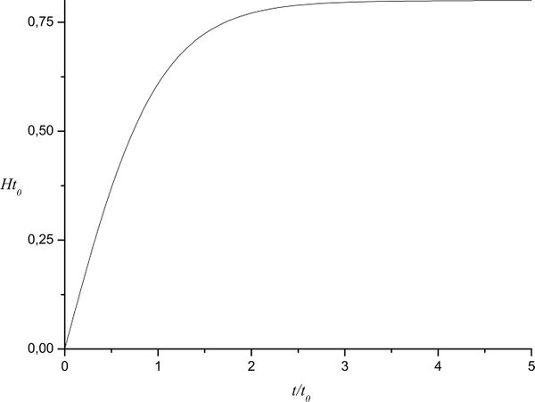
Time dependence of the Hubble parameter (in units of the age of the Universe).

Problem 25
Find time dependence of dark matter density.
Present the first Friedmann equation in the form \[\rho_m=\frac{1}{8\pi G}(3h^2-\Lambda)\] and make use of results of the previous problem to obtain \[\rho_m=\frac{\Lambda}{8\pi G}\frac{1}{\sinh^2(t/t_\Lambda)}.\]
Problem 26
Find the asymptotic (in time) value of the Hubble parameter.
The required asymptote can be obtained in two ways: first, from the time dependence of the Hubble parameter (see the previous problem), and second, immediately from the first Friedmann equation in the SCM. Taking into account that $\rho_{m} \to 0$ at $t\to \infty$, one gets $$ H_{\infty} = \frac{2}{3t_\Lambda} = \sqrt {\frac{\Lambda}{3}}. $$
Problem 27
At present the age of the Universe $t_0\simeq13.7\cdot10^9$ years is close to the Hubble time $t_H=H_0^{-1}\simeq14\cdot10^9$ years. Does the relation $t^*\simeq t_H(t^*)=H^{-1}(t^*)$ for the age $t^*$ of the Universe hold for any moment of its evolution
This relation cannot be satisfied in arbitrary moment of time, as the Hubble parameter has limit value in the SCM (see the previous problem): $$ \frac{t^*}{t_H(t^*)} = H\left( t^*\right)t^* = \frac{2}{3}\frac{Arcth\sqrt {\Omega _\Lambda(t^*)}}{\sqrt{\Omega_\Lambda (t^*)}}. $$ For $t\to \infty,\;\Omega _\Lambda\left( t^* \right) \to 1,$ and $$\frac{t^*}{t_H(t^*)} \to \infty. $$ \item {\bf Determine values of state parameter for the dark energy, that provide accelerated expansion of Universe in the present time.} $$ \begin{gathered} \sum\limits_i (\rho _{i0} + 3p_{i0}) < 0\; \Rightarrow \rho _{m0} + \rho _{DE0} + 3w_{DE}\rho _{DE0} < 0; \\ w_{DE} < - \frac{1}{3}\left( 1 + \frac{\Omega _{m0}}{\Omega _{DE0}}\right); \\ w_{DE} < - \frac{1}{3}\Omega _{DE0}^{-1};\; w_{DE} < - 0.46\\ \end{gathered} $$
Problem 28
Find current value of the deceleration parameter.
For a multi-component system the deceleration parameter equals to $$ q = \frac{\Omega}{2} + \frac{3}{2}\sum\limits_i {w_i}\Omega _i $$ In the SCM $\Omega = 1,w_m = 0,\;w_\Lambda= - 1,$ and $$ \begin{gathered} q = \frac{1 - 3\Omega_{\Lambda 0}}{2};\\ q_0 \simeq - 0.6 \\ \end{gathered} $$
Problem 29
Find the redshift dependence of the deceleration parameter. Analyze the limiting cases.
$$ \begin{gathered} q \equiv - \frac{a\ddot a}{\dot a^2} = - \frac{\ddot a}{a}\frac{1}{H^2}; \\ \frac{\ddot a}{a} = - \frac{4\pi G}{3}\sum\limits_i \left( \rho _i + 3p_i \right) = - \frac{1}{2}H_0^2\sum\limits_i \Omega _{i0}\left(1 + 3w_i\right)(1 + z)^{3\left(1 + w_i\right)} ; \\ H^2 = H_0^2\sum\limits_i \Omega _{i0}(1 + z)^{3\left( 1 + w_i \right)}; \\ q = \frac{3}{2}\frac{\sum\limits_i \Omega _{i0}\left( 1 + w_i \right)(1 + z)^{3\left( 1 + w_i \right)}} {\sum\limits_i \Omega _{i0}(1 + z)^{3\left( 1 + w_i\right)} } - 1 \\ \end{gathered} $$ In the SCM $$ q = \frac{1}{2}\frac{\Omega _{m0}(1 + z)^3- 2\Omega _{\Lambda 0} } {\Omega _{m0}(1 + z)^3+\Omega_{\Lambda 0}} $$ $$ q(z \to \infty ) = \frac{1}{2},\;q(z \to - 1) = - 1 $$
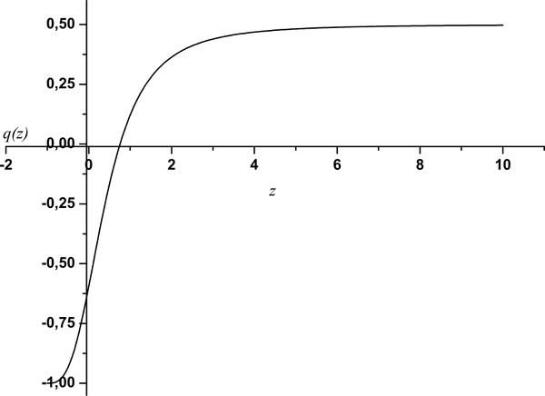
Dependence of the deceleration parameter on the redshift.

Problem 30
Find and plot the time dependence of the deceleration parameter.
$$ \begin{gathered} q = - \frac{\ddot aa} {\dot a^2} = - \frac{\ddot a} {aH^2}; \\ a(t) = A^{1/3}sh^{2/3}\left(t/{t_\Lambda}\right);\quad A\equiv \frac{\Omega_ {m0}} {\Omega _{\Lambda 0}}; \\ \frac{t_0} {t_\Lambda } = Arth\sqrt {\Omega _{\Lambda 0}} ;\quad H = \frac{2} {3}\frac{1} {t_\Lambda }cth\left( \frac{t} {t_\Lambda }\right); \\ q = \frac{1} {2}\left[ 1 - 3th^2\left( \frac{t} {t_\Lambda }\right)\right] \\ \end{gathered} $$
Problem 31
Find the moment of time when the dark energy started to dominate over dark matter. What redshift did it correspond to?
$$ \begin{gathered} \left( \frac{\dot a}{a} \right)^2 = \frac{8\pi G} {3}\rho _{cr}\left( \Omega _{m0}(1 + z)^3+\Omega_{\Lambda 0}\right); \\ \Omega _{m0}(1 + z^*)^3 =\Omega _{\Lambda 0};\\ z^* = \left(\frac{\Omega _{\Lambda 0}} {\Omega _{m0}}\right)^{1/3}-1; \\ \Omega _{\Lambda 0}\simeq 0.73;\quad \Omega _{m0}\simeq 0.27; \\ z^* \simeq 0.39; \\ \Omega _\Lambda = th^2\left(\frac{t} {t_\Lambda }\right);\quad \Omega _m = 1 - \Omega _\Lambda = ch^{-2}\left( \frac{t} {t_\Lambda } \right); \\ \Omega _\Lambda(\tilde t) = \Omega _m(\tilde t) \to \tilde t = \frac{Arsh(1)}{Arth(\sqrt {\Omega _{\Lambda 0} })}t_0 \simeq 9.5\cdot10^9 \,years \\ \end{gathered} $$
Problem 32
Determine the moment of time and redshift value corresponding to the transition from decelerated expansion of the Universe to the accelerated one.
$$ \begin{gathered} \frac{\ddot a} {a} = \frac{4\pi G} {3}\rho_{cr}\left[2\Omega_{\Lambda 0} - \Omega _{m0}(1 + z)^3\right]; \\ 2\Omega _{\Lambda 0} = \Omega _{m0}(1 + z^*)^3; \\ z^* = \left( \frac{2\Omega_{\Lambda 0}} {\Omega _{m0}}\right)^{1/3} - 1; \\ \Omega _{\Lambda 0}\simeq 0.73;\quad \Omega _{m0}\simeq 0.27; \\ z^* \simeq 0.745 \\ \end{gathered} $$ Let us now determine the time moment $t^*$ of the transition $$ \begin{gathered} a^* = \frac{1} {1 + z^*} = \left(\frac{\Omega _{m0}} {2\Omega _{\Lambda 0}} \right)^{1/3}; \\ t(a) = \frac{2}{3\sqrt{\Omega_{\Lambda 0}}H_0}Arsh\left(\sqrt{ \frac{\Omega_{\Lambda 0}} {\Omega_{m0}}}a^{3/2} \right); \\ t^* = \frac{2} {3\sqrt {\Omega _{\Lambda 0}}}H_0Arsh\left(\sqrt {1/2} \right) \\ \end{gathered} $$ There is an alternative way to solve the problem. In the multi-component Universe with the corresponding state equations $p_i = w_i\rho _i$ the deceleration parameter $q \equiv - \frac{\ddot aa}{\dot a^2}$ equals to $$ q = \frac{\Omega } {2} + \frac{3} {2}\sum\limits_i w_i\Omega _i $$ In the case of the SCM $\Omega =1$ and $$ q = \frac{1} {2} - \frac{3} {2}\frac{\Omega _{\Lambda 0}} {\left[\left(1 + z\right)^3\Omega _{m0}+\Omega_{\Lambda 0}\right]} $$ From the condition $q=0$ it follows that $$ z^* =\left(\frac{2\Omega_{\Lambda 0}} {\Omega _{m0}} \right)^{1/3}- 1 $$ For $\Omega _{\Lambda 0} = 0.73,\;\Omega _{m0} = 0.27$ one obtains that $$ z^* = 0.745 $$
Problem 33
Solve the previous problem using the derivative $d\eta/d\ln a$.
$$ \frac{d\eta} {d\ln a} = a\frac{dt}{ada} = \frac{1}{aH} = \frac{1}{\dot a} $$ If the quantity $aH = \dot a$ grows, then $\ddot a > 0,$ which corresponds to the accelerated expansion (inflation) of the Universe. In the SCM the quantity $$ \frac{aH}{H_0} \simeq \sqrt{ \frac{0.27 + 0.73a^3}{a}} $$ starts to grow at $a=0.573,$ which corresponds to $z=0.745$
Problem 34
Is dark energy domination necessary for transition to the accelerated expansion?
No. The transition to the accelerated expansion takes place at $(z=0.75)$, which is considerably earlier than the transition to the dark energy domination stage at $(z=0.45).$
Problem 35
Consider flat Universe composed of matter and dark energy in form of cosmological constant. Find the redshift value corresponding to equality of densities of the both components $\rho_m(z_{eq})=\rho_\Lambda(z_{eq})$ and the one corresponding to beginning of the accelerated expansion $q\left(z_{accel} \right) = 0$. Obtain relation between $z_{eq}$ and $z_{accel}$.
$$ \begin{gathered} z_{eq} = \left(\frac{\Omega _\Lambda} {\Omega _{m0}} \right)^{1/3}- 1; \\ z_{accel}= \left(\frac{2\Omega_\Lambda } {\Omega _{m0}}\right)^{1/3}- 1; \\ z_{accel} = 2^{1/3}\left(z_{eq}+ 1\right) - 1 \\ \end{gathered} $$
Problem 36
Show that density perturbations stop to grow after the transition from dust to $\Lambda$-dominated era.
On the $\Lambda$-dominated stage the non-relativistic matter density perturbation size depends on conformal time as \begin{equation}\label{1SCM30} a(\eta)=-\frac{1}{H\eta}, \,\, \eta=-const\cdotp e^{-Ht},\,\,\eta<0 \end{equation} where the Hubble parameter $H$ is constant, $H^2=(8\pi/3)G\rho_\Lambda$. The linearized Einstein equations for the case of single-component medium take the following form in the momentum representation: \begin{equation}\label{3SCM30} k^2\Phi+3\frac{a^{'}}{a}+3\frac{a^{'2}}{a^2}\Phi=-4\pi Ga^2\delta\rho, \end{equation} \begin{equation}\label{2SCM30} \Phi^{''}+3\frac{a^{'}}{a}\Phi^{'}+\left(2\frac{a^{''}}{a} - \frac{a^{'2}}{a^2}\right)\Phi=4\pi Ga^2\delta p. \end{equation} Assuming that the $\Lambda$-term is constant (which is exactly true for the vacuum energy density) one obtains $\delta\rho_\Lambda=\delta p_\Lambda=0$. Using \eqref{2SCM30} and taking into account \eqref{1SCM30} we come up with the equation: $${\Phi}^{''}-\frac{3}{\eta}{\Phi}^{'}-\frac{3}{\eta^2}\Phi=0,$$ Solutions of the equation behave as $$\Phi\propto\eta\propto\frac 1a$$ and $$\Phi\propto\eta^3\propto\frac{1}{a^3}.$$ Use now \eqref{3SCM30} for the modes beyond the horizon and take into account that for dust density $\rho_M\propto a^{-3}.$ Keeping only the first solution for the gravitational potential (the second decays too fast), one can see that the density perturbations do not grow: for the modes under horizon the relation $$\delta_M\propto a^3\frac{k^2}{a^2}\Phi=const$$ holds. Therefore the perturbations stop to grow at the transition from the dust-dominated to the $\Lambda$-dominated stage. If the present accelerated expansion of the Universe is actually caused by non-zero cosmological constant, then the structure formation from small primary perturbations is eventually close to end and it will never resume again: the structures larger than the presently observed ones will never appear.
Problem 37
What happens to the velocity fluctuations of non-relativistic matter and radiation with respect to Hubble flow in the epoch of cosmological constant domination?
Problem 38
Find the ratio of baryon to non-baryon components in the galactic halo.
Problem 39
Imagine that in the Universe described by SCM the dark energy was instantly switched off. Analyze further dynamics of the Universe.
Problem 40
Estimate density of dark energy in form of cosmological constant using the Hubble diagram for the neighborhood of the Local group.
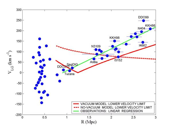
Hubble diagram for the neighborhood of the Local group.

An elegant and simple method was recently proposed (see A.D.Chernin, UFN 178, 267 (2008)), which allows not only to become convinced in the existence of the dark energy but also to estimate its density. The method is based on the assumption, that the dark energy (in form of the cosmological constant) governs the Hubble flow even on comparably small distances $\left( \sim \,Mpc \right)$. Consider the resulting force $\vec{F}$ (per unit mass), acting on a galaxy from the picture \ref{hubble_diagram}. The force is a sum of two contributions: $$ \vec{F}=\vec{F}_N+\vec{F}_\Lambda $$ Here $\vec{F}_N$ is the force produced by the total mass of the Local group, and $F_{\Lambda }$ is the force created by the dark energy. For a crude estimate let us neglect the non-spherical mass distribution in the Local group. Then the force acting on a satellite galaxy in a given point $R$ outside the local Group equals to $$ F=-\frac{GM_{LG}}{R^2}+\frac{8\pi G}{3}{\rho_{\Lambda }}R, $$ where $M_{LG}\simeq (1\div 3) \times 10^{12}M_{\odot }$ is the total mass of the Local group. As can be seen from the picture, the transition from domination of the local group gravity to the vacuum domination takes place on the distance of order $R_{0}=1.8\div 2\; \, Mpc.$ It allows to make a rough estimate of the dark energy density from the condition $F\left( R=R_0 \right)=0.$ The estimate results in the following $$ (0.1\pm 0.03)<\rho_V<(1\pm 0.3)\times 10^{-26} \, kg/m^3. $$ The proximity of the obtained crude estimate to the actual value of the dark energy density in the SCM is striking. $$ \rho_{V}\simeq (0.75\pm 0.05)\times 10^{-26}\, kg/m^3. $$
Problem 41
Estimate the Local group mass by methods used in the previous problem.
Problem 42
Find "weak" points in the argumentation of the two preceding problems.
Problem 43
The product of the age of the Universe and current Hubble parameter (the Hubble's constant) is a very important test (Sandage consistency test) of internal consistency for any model of Universe. Analyze the parameters on which the product $H_0 t_0$ depends in the Big Bang model and in the SCM.
Problem 44
Show that for a fixed source of radiation the luminosity distance for high redshift values in flat Universe is greater for the dark energy dominated case compared to the non-relativistic matter dominated one.
In the case of Universe filled by dark energy and non-relativistic matter, the photometric distance is equal to
$$
d_L = \frac{1 + z}
{H_0}\int_0^z \frac{dz'}
{\sqrt{\Omega _{m0}\left(1 + z'\right)^3+ \Omega _{DE0}\left(1 + z' \right)^{3\left( 1 + w_{DE}\right)}}}
$$
In the case $\Omega _{m0} = 1,\;\Omega _{DE0} = 0$
one obtains
$$
d_L = \frac{2}
{H_0}\left[1 + z -(1 + z)^{1/2}\right]
$$
and in the case $\Omega _{m0} = 0,\;\Omega _{DE0} = 1$
$$
d_L = \frac{1}{H_0}z(1 + z)
$$
instead.
In means that the supernova appear dimmer in the dark energy dominated Universe.
Problem 45
In the observations that discovered the accelerated expansion of the Universe the researchers in particular detected two $Ia$ type supernovae: $1992P$, $z=0.026$, $m=16.08$ and $1997ap$, $z=0.83$, $m=24.32$. Show that these observed parameters are in accordance with the SCM.
The apparent $m$ and absolute $M$ stellar magnitudes are related with the photometric distance $d_L$ by the expression \begin{equation}\label{p(1)} m - M = 5\log _{10}\left(\frac{d_L} {\mbox{Mpc}} \right) + 25 \end{equation} The photometric distance in the SCM is equal to \begin{equation}\label{p(2)} d_L = \frac{1 + z} {H_0}\int_0^z \frac{dz'} {\sqrt {\Omega _{m0}(1 + z)^3 + \Omega _\Lambda}} \end{equation} For small $z$ $d_L(z) \simeq z/H_0.$ Using the supernova $1992P$ with small $z=0.026$ one can find $M = - 19.09.$ Assuming that the $1a$-type supernova are standard candles (they have equal absolute magnitudes), one obtains from the relation \ref{p(1)} supernova with $z=0.83$ $$H_0d_L\simeq 1.16$$ From the other hand it follows from the relation \ref{p(1)} that in the case $\Omega _{m0} = 1,\;\Omega_\Lambda = 0$ $$ H_0d_L\simeq 0.95 $$ In the SCM one gets much better agreement: $$ H_0d_L \simeq 1.2 $$
Problem 46
Find the redshift value, at which a source of linear dimension $d$ has minimum visible angular size.
The apparent angular size equals to $$\delta \theta = {{(1 + z)^2 d } \over {d_L (z)}},$$ where $d_L (z)$ is the photometric distance from a source with the redshift $z$. In the case of cosmological constant domination the photometric distance is: $$d_L (z) = - {z \over {H_0 \Omega _\Lambda ^{1/2} }},$$ In the SCM (see the previous problem) $$ d_L = \frac{1 + z} {H_0}\int_0^z \frac{dz'} {\sqrt {\Omega _{m0}(1 + z)^3 + \Omega _\Lambda}} $$ then the angular size is $$\delta \theta = - {{H_0 \Omega _\Lambda ^{1/2} d} \over 2}{{(1 + z)^2 } \over z},$$ and $z = - 1$. It corresponds to infinitely far future.
Problem 47
Compare the observed value of the dark energy density with the one expected from the dimensionality considerations (the cosmological constant problem).
The dimensionality considerations suggest the following value for density of the dark energy in form of the cosmological constant \[\rho_\Lambda^{(dim)}\sim M_{Pl}^4\approx10^{76}GeV^4.\] At the same time the observed value fixed by the SCM is \[\rho_\Lambda^{(obs)}\approx10^{-48}GeV^4.\] This huge disagreement \[\frac{\rho_\Lambda^{(dim)}}{\rho_\Lambda^{(obs)}}>10^{120}\] is called the cosmological constant problem. It presents a fundamental problem for elementary particles theory and physics in general, rather than for cosmology itself. (Look for details in R.Bousso, TASI Lectures on the cosmological constant)
Problem 48
Determine the density of vacuum energy using the Planck scale as cutoff parameter.
For a quantum field with a given mode of frequency $\omega$, the zero-point energy is $\pm\omega/2$ with the plus sign for a bosonic field and the minus sign for a fermionic field. The total zero-point energy is then $\pm\sum\limits_i\omega_i/2$. In the continuum limit, we have for a free field (bosonic or fermionic) \[\frac12\sum\limits_i\omega_i=\frac12\int\frac{d^3xd^3k}{(2\pi)^3}(k^2+m^2)^{1/2}=V\int\frac{k^2dk}{4\pi^2}(k^2+m^2)^{1/2}.\] This integral diverges, thus we need to introduce the physical cutoff. In cosmological context this cutoff must be the Planck mass at largest. With the cutoff $k_{max}\sim M_{Pl}$ one obtains \[\rho_\Lambda=\int_0^{k_{max}}\frac{k^2dk}{4\pi^2}(k^2+m^2)^{1/2} \approx\frac{k_{max}^4}{16\pi^2}=\frac{M_{Pl}^4}{16\pi^2} \approx10^{74}GeV^4.\] This result only slightly modifies the dimensional considerations given in the previous problem.
Problem 49
Identifying the vacuum fluctuations density with the observable dark energy value in SCM, find the required frequency cutoff magnitude in the fluctuation spectrum.
\[\nu_{max}=10^{12}Hz.\]
Problem 50
What purely cosmological problem originates from the divergence of the zero-point energy density?
If the zero-point energy density is infinite, then our Universe is infinitely curved and the space size is infinitely small.
Problem 51
With exact supersymmetry, the bosonic contribution to cosmological constant is canceled by its fermionic counterpart. However, we know that our world looks like not supersymmetric. Supersymmetry, if exists, has to be broken above or around $100GeV$ scale. Compare the observed value of the dark energy density with the one expected from broken supersymmetry.
If we take the $k_{max}^{(SUSY)}\sim100GeV$ cutoff, then \[\rho_\Lambda^{(SUSY)}=\frac{\left(k_{max}^{(SUSY)}\right)^4}{16\pi^2}\approx10^6GeV^4.\] \[\frac{\rho_\Lambda^{(SUSY)}}{\rho_\Lambda^{(obs)}}>10^{54}.\] Thus supersymmetry does not solve the problem of the cosmological constant.
Problem 52
Determine duration of the inflation period.
Let us see what happens with the relative density during all the history of Universe. From the first Friedmann equation it follows that in the matter-dominated epoch $\left| \Omega - 1 \right| \sim t^{2/3},$ and in the radiation-dominated epoch $\left| \Omega - 1 \right| \sim t^{2/3}.$ Then assume that inflation started at $t_i,$ and finished at $t_f.$ Then in the period of $t_f < t < t_{eq} = 50000$ years the radiation dominated and the range $t_{eq} < t < t_0 $ corresponds to the matter domination epoch. Then the presently observed difference $$ \left|\Omega (t_0 ) - 1 \right| = \left| \Omega (t_i ) - 1 \right|e^{ - 2H(t_f - t_i )} \left( \frac{t_{eq} } {t_f } \right)\left( \frac{t_0} {t_{eq} }\right)^{2/3} $$ According the SCM $\left|\Omega \left( t_0\right) - 1 \right| < 0.04.$ If one assumes that before the beginning of the inflation there was $\left|\Omega \left( t_i \right) - 1 \right| \sim 1,$ then $$ N > \frac{1}{2}\ln \left[\frac{\Omega \left( t_i \right) - 1}{\Omega \left(t_0\right) - 1}\left( \frac{t_{eq}}{t_f } \right)\left( \frac{t_0}{t_{eq}} \right)^{2/3} \right] \approx 60 $$ Assume that radiation dominated before the inflation started. Then $H = \frac{1}{2t}.$ If at the moment of time $t_i$ the vacuum dark energy started to dominate and then the expansion continued with constant rate, then $H\approx 1/t_i$ during the inflation. And finally one obtains that $$ N = H\left(t_f - t_i\right) \approx \frac{t_f - t_i } {t_i } $$ it is commonly assumed that the inflation finishing time is of order of the Grand Unification time $t_f\approx 10^{-35}.$ Therefore $t_f\approx 10^{-38}.$ Evidently the inflation could last longer as we used only lower estimate for $N.$
Problem 53
Plot the dependence of luminosity distance $d_L$ (in units of $H_0^{-1}$) on the redshift $z$ for the two-component flat Universe with non-relativistic liquid ($w=0$) and cosmological constant
($w=-1$). Consider the following cases:
a) $\Omega_\Lambda^0=0$;
b) $\Omega_\Lambda^0=0.3$;
c) $\Omega_\Lambda^0=0.7$;
d) $\Omega_\Lambda^0=1$.
Problem 54
For a Universe filled by dark energy with state equation $p_{DE}=w_{DE}\rho_{DE}$ and non-relativistic matter obtain the Taylor series for $d_L$ in terms of $z$ near the observation point $z_0=0$. Explain the obtained result.
In the universe filled by dark energy with the state equation $p_{DE}=w_{DE}\rho_{DE}$ and non-relativistic dark matter the photometric distance takes on the form: \begin{equation} \label{d_L} d_L = \frac{1 + z} {H_0}\int_0^z \frac{dz'} {\sqrt{\Omega _{m0}\left(1 + z'\right)^3+ \Omega _{DE0}\left(1 + z' \right)^{3\left( 1 + w_{DE}\right)}}} \end{equation} Expand the integrand in Taylor series in $z$ in vicinity of the observation point $z_0=0$ to obtain $$ \begin{gathered} \label{tey} \frac{1}{\sqrt{\Omega _{m0}\left(1 + z'\right)^3+ \Omega _{DE0}\left(1 + z' \right)^{3\left( 1 + w_{DE}\right)}}}\simeq \\ \simeq 1 -\frac{3}{2}\left(1+w_{DE}\Omega _{DE0}\right)z+\frac{3}{4}\left(3w_{DE}\Omega _{DE0}-1\right)z^2.\nonumber \end{gathered} $$ Substitution of the decomposition (\ref{tey}) into the integral (\ref{d_L}) results in the following: \begin{equation} \label{d_L1} d_L = \frac{1 + z} {H_0}\left(z -\frac{3}{4}\left(1+w_{DE}\Omega _{DE0}\right)z^2+\frac{1}{4}\left(3w_{DE}\Omega _{DE0}-1\right)z^3\right). \end{equation}
Problem 55
Determine position of the first acoustic peak in the CMB power spectrum produced by baryon oscillations on the surface of the last scattering.
Early Universe was filled by photon-baryon plasma, which can be treated as a single-component liquid. The baryons were trapped by the potential walls generated by density fluctuations, and they were eventually compressed. The contraction lead to heating of the plasma and therefore to increasing radiative pressure of the photons which is directed outside. Finally the radiative pressure stop the compression and lead to expansion of the plasma. During the expansion the plasma cools down and its radiative pressure decreases. The gravity starts to dominate again leading to repeated compression. The concurrence between the gravity and the pressure lead to longitudinal (acoustic) oscillations in the photon-baryon fluid. When the matter and the radiation get decoupled in the recombination process, the picture of the acoustic oscillations remains frozen into the CMB. Today we detect the evidence of the primordial acoustic waves (dense and diluted regions) in form of the primary anisotropy in the CMB.
It is well known that any acoustic wave, whatever complicatedly shaped, can be represented in form of superposition of modes with different wave numbers $k$, $k\propto 1/\lambda $. Every mode $\lambda $ corresponds to certain angular scale $\theta $ on the sky. Therefore in order to facilitate the comparison of the theory with observations, one should use the angular (multipole) decomposition in terms of the Legendre polynomials $P_{l} (\cos \theta )$, instead of the Fourier transform in terms of sines and cosines. Order of the polynomial $l$ plays the same role as the index $k$ in the Fourier decomposition. For $l\ge 2$ the Legendre polynomials are oscillating functions in the interval $\left[1,-1\right]$. Number of the oscillations increases with growth of $l$. Therefore
\begin{equation} \label{acust1_}
l\propto \frac{1}{\theta }
\end{equation}
The temperature fluctuations can be observed and qualitatively analyzed with help of paired measurements in the directions $\stackrel{\frown}{n},\stackrel{\frown}{n}'$, so that $\stackrel{\frown}{n}\cdot \stackrel{\frown}{n}'=\cos \theta $. Taking average over all the pairs in the assumptions of Gaussian fluctuations, one obtains the two-point correlator $C(\theta )$, which can be presented in terms of the multipole decomposition
\begin{equation} \label{acust2_}
\left\langle \delta T(\stackrel{\frown}{n})\cdot \delta T(\stackrel{\frown}{n}')\right\rangle \equiv C(\theta )=\sum _{l}\frac{2l+1}{4\pi } C_{l} P_{l} (\cos \theta )
\end{equation}
where $C_{l} $ are the coefficients.
As we already mentioned, the analysis of the temperature fluctuations enables us to clarify the structure of the longitudinal oscillations. The mode with the maximum wavelength corresponds to the maximum angular size of the primary anisotropy. This fundamental mode was detected the first. There are reliable evidences of the fact that the second and the third modes were also already detected. The distance $r_{s} $, passed by the acoustic wave during the time period before the recombination, is called the sound horizon. The sound horizon is fixed by (or rather fixes) the physical scale o the last scattering surface. Size of the sound horizon depends on values of the physical parameters. Distance to the last scattering surface $d_{sls} $ depends on the cosmological parameters too. Together they determine the angular size of the sound horizon$\theta _{s} $ (see Fig.)
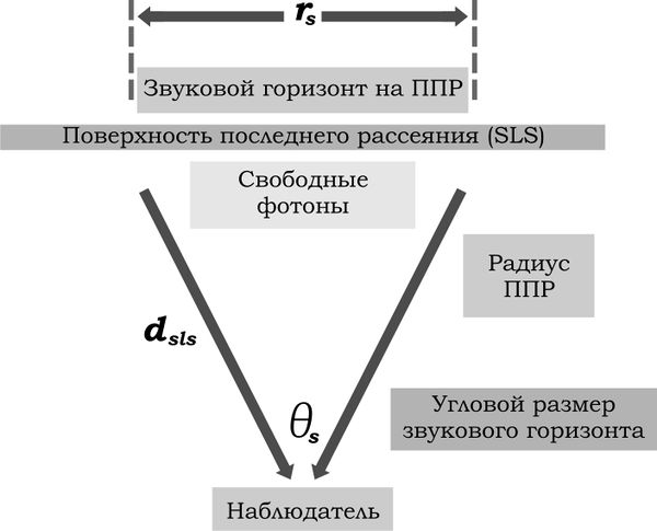
Dependence of the deceleration parameter on the redshift.

\begin{equation} \label{acust3_}
\theta _{s} \approx \frac{r_{s} }{d_{sls} }
\end{equation}
Analysis of the temperature anisotropy allows to determine $\theta _{s} $. Varying the cosmological parameters in $r_{s} ,d_{sls} ,$ one achieves the best agreement with the observations and thus fixes the cosmological parameters.
We can estimate the sound horizon size as the length passed by sound from the moment $t=0$ to the recombination time $t_{*} $
\begin{equation} \label{acust4_}
r_{s} (z_{*} ;\Omega _{b} ,\Omega _{r} )\approx \int _{0}^{t_{*} }c_{s} dt
\end{equation}
where $z_{*} $ is the redshift of the recombination moment $\left(z_{*} \approx 1100\right)$, $c_{s} $ is the sound speed in the photon-baryon medium
\begin{equation} \label{acust5_}
c_{s} \approx c\left[3\left(1+\frac{3\Omega _{b} }{\Omega _{r} } \right)\right]^{-1/2}
\end{equation}
To determine $dt$ one should use the first Friedmann equation in the form
\begin{equation} \label{acust6_}
\left(\frac{da}{dt} \right)^{2} =H_{0}^{2} \left[\Omega _{r0} \left(\frac{a_{0} }{a} \right)^{2} +\Omega _{m0} \frac{a_{0} }{a} +\Omega _{k0} +\Omega _{\Lambda 0} \left(\frac{a}{a_{0} } \right)^{2} \right]
\end{equation}
Making use of the relations $\frac{a_{0} }{a} =1+z$ and $\Omega _{r} +\Omega _{m} +\Omega _{\Lambda } +\Omega _{k} =1$, one obtains
\begin{equation} \label{acust7_}
dt=H_{0}^{-1} (1+z)^{-1} \left\{\left(1+z\right)^{2} \left(1+\Omega _{m,0} z\right)+z(z+2)\left[\left(1+z)^{2} \Omega _{r.0} -\Omega _{\Lambda ,0} \right)\right]\right\}^{-1/2} dz
\end{equation}
Distance to the last scattering surface, which corresponds to its angular size, is determined by the quantity called the angular diameter distance. It is connected by the photometric distance $d$ by the simple relation
\begin{equation} \label{acust8_}
d_{sls} =\frac{d}{(1+z_{*} )^{2} }
\end{equation}
The position of the first acoustic peak is determined by
\begin{equation} \label{acust9_}
l\approx \frac{d_{sls} }{r_{s} }.
\end{equation}
Let us now predict the position of the first peak for the case of flat Universe. To the leading order the sound speed is
\[c_{s} =\frac{c}{\sqrt{3} }. \]
Let us assume also that in the recombination epoch the Universe was matter-dominated. Under such assumptions one gets
\begin{equation} \label{acust10_}
r_{s} =\frac{c_{s} }{H_{0} \sqrt{\Omega _{m} } } \int _{z_{*} }^{\infty }(1+z)^{-5/2} dz =r_{s} =\frac{2c_{s} }{3H_{0} \sqrt{\Omega _{m} } } \left(1+z_{*} \right)^{-3/2}
\end{equation}
Using the standard procedure (see section 4), we obtain for the comoving radial coordinate $r_{sls} $ of the last scattering surface the following
\begin{equation} \label{acust11_}
r_{lsr} =\frac{c}{H_{0} } \int _{0}^{z_{*} }\left[\Omega _{m} (1+z)^{^{3} } +\Omega _{\Lambda } \right] ^{-1/2} dz
\end{equation}
Replacing the integrand by its binomial decomposition
\[\Omega _{m}^{-1/2} (1+z)^{-3/2} -\left(\Omega _{\Lambda } /2\Omega _{m}^{3/2} \right)\left(1+z\right)^{-9/2} \]
and taking into account that
\[d_{sls} =r_{sls} /(1+z_{*} ),\]
we obtain
\begin{equation} \label{acust12_}
d_{sls} =\frac{2c}{7H_{0} (1+z_{*} )} \left\{7\Omega _{m}^{-1/2} -2\Omega _{\Lambda } \Omega _{m}^{-3/2} +{\rm O} \left[\left(1+z_{*} \right)^{-1/2} \right]\right\}.
\end{equation}
Using the relation $\Omega _{\Lambda } =1-\Omega _{m} $ and neglecting the higher order terms, one obtains
\begin{equation} \label{acust13_}
d_{sls} \approx \frac{2c\Omega _{m}^{-1/2} }{7H_{0} (1+z_{*} )} \left(9-2\Omega _{m}^{3} \right)
\end{equation}
Combination of the relations \eqref{acust10_} and \eqref{acust13_} gives for the first acoustic peak the following
\begin{equation} \label{acust14_}
l\approx \frac{d_{sls} }{r_{s} } \approx 0.74\sqrt{1+z_{*} } \left(9-2\Omega _{m}^{3} \right)\simeq 220.
\end{equation}
Problem 56
\bf Compare the asymptotes of time dependence of the scale factor $a(t)$ for the SCM and de Sitter models. Explain physical reasons of their distinction.
Problem 57
Redshift for any object slowly changes due to the acceleration (or deceleration) of the Universe expansion. Estimate change of velocity in one year.
$$ \Delta z = \dot z \Delta t = H_0 \left(1 + z - {H(z)\over H_0} \right)\Delta t $$ $$H(z)=H_0 \left[\Omega_{m0}(1+z)^3+\Omega_{\Lambda 0}\right]^{1/2}$$ $$\Omega_{m0}+\Omega_{\Lambda 0}=1,~\Omega_{m0}\approx 0.3$$ $$\Delta z \approx 2\cdot 10^{-11}$$ $$\Delta v = c{\Delta z\over 1+z}\approx 0.25~\mbox{cm/s}$$
Problem 58
Determine the lower limit of ratio of the total volume of the Universe to the observed one?
If the Universe is the 3-sphere, then its radius is $R_0=a_0$ $$ R_0 = \frac{1}{H_0 \sqrt {\left| \Omega _{curv} \right|} } $$ For the SCM parameters the cosmological horizon equals to $$ L_{p,0} = a_0 \int_0^{t_0 } \frac{dt}{a(t)} = \frac{3.6}{H_0} $$ We assumed that $a(t)\sim t^{2/3}.$ Therefore $$ \frac{R_0} {L_{p,0} } = \frac{1} {3.6\sqrt {\left| \Omega _{curv}\right|} } $$ Taking into account that $\left|\Omega _{curv} \right| < 0.02,$ one obtains $\frac{a_0}{L_{p0} } > 2$. Number of the regions similar to the one inside our horizon equals to the ratio of the 3-sphere volume $2\pi ^2 a_0^3 $ to the volume of the observed Universe $$ N = \frac{2\pi ^2 a_0^3} {(4\pi /3)L_{p0}^3 } \simeq 4.7\left(\frac{a_0 } {L_{p0} } \right)^3 > 38 $$ Thus we can see not more than $3 \%$ of the Universe volume.
Problem 59
What is the difference between the inflationary expansion in the early Universe and the present accelerated expansion?
The difference is in the fact that in the present time there is about $27 \%$ of non-relativistic matter which was absent in the inflation period. The numerical values of Hubble parameter in the beginning of the inflation was very different from the one at the beginning of the current period of accelerated expansion of Universe.
Problem 60
Compare the values of Hubble parameter at the beginning of the inflation period and at the beginning of the present accelerated expansion of Universe.
$$ h^2 (x) = \Omega _{m0} x^3 + (1 - \Omega _{m0} )x^\alpha ;\quad \alpha = 3(1 + w) $$ Assume for simplicity that the Universe is spatially flat. From the definition $O(x)$ it follows that $$ O(x) = \Omega _{m0} + \left( 1 - \Omega _{m0}\right)\frac{x^\alpha - 1} {x^3 - 1} $$ The required result follows from the fact that $\alpha =0$ for cosmological constant, $\alpha >0$ for quintessence and $\alpha <0$ for phantom energy.
Problem 61
Plot the dependencies $h(x)=H(x)/H_0(x)$, where $x=1+z$, in the SCM, for quintessence and for phantom energy cases.
Plots of the dependencies $ h(x) = H(x)/H_0 (x);\quad x = 1 + z $ in the SCM are presented on Fig. \ref{fig:52} for phantom energy and quintessence.
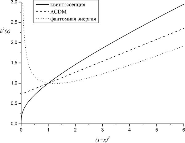
Dependence of the deceleration parameter on the redshift.

Problem 62
Find the constraints imposed by the Weak Energy Condition (WEC) for the dark energy on the redshift-dependent Hubble parameter. (Inspired by A.Sen, R.Scherrer)
The redshift-dependent Hubble parameter $H(z)$ is defined by \[H^2(z)=\frac{8\pi G}{3}(\rho_m+\rho_{DE})\] This equation can be rewritten as \begin{equation}\label{SCM_eq_76_1} E^2(z)\equiv\frac{H^2(z)}{H^2_0(z)}=\Omega_{m0}(1+z)^3+(1-\Omega_{m0})\frac{\rho_{DE}}{\rho_{DE0}} \end{equation} The WEC forces \[\frac{\rho_{DE}}{\rho_{DE0}}\ge1 \ \left(\frac{d\rho}{dz}\ge0\right)\] for $z>1$, so equation (\ref{SCM_eq_76_1}) becomes \begin{equation}\label{SCM_eq_76_2} E^2(z)\ge\Omega_{m0}(1+z)^3+(1-\Omega_{m0}) \end{equation} Going back to equation (\ref{SCM_eq_76_2}) and taking the derivative with respect to $z$ (which we denote throughout with a prime) gives: \[ 2E(z)\frac{dE}{dz}=3\Omega_{m0}(1+z)^2+\frac{1-\Omega_{m0}}{\rho_{DE0}}\frac{d\rho_{DE}}{dz}. \] Now the WEC implies that \[\frac{d\rho_{DE}}{dz}\ge0,\] so we get \begin{equation}\label{SCM_eq_76_3} E(z)\frac{dE}{dz}\ge\frac32\Omega_{m0}(1+z)^2. \end{equation} Equations (\ref{SCM_eq_76_2}) and (\ref{SCM_eq_76_3}) give the constraints that the WEC for the dark energy places on the redshift-dependent Hubble parameter.
Problem 63
Using the statefinders, show that the power law cosmology mimics SCM model at (see Chapters 3 and 9)
Recall that the statefinders are defined as \[r\equiv\frac{\dddot a}{aH^3},\ s\equiv\frac{r-1}{3(q-1/2)}, \ q\ne\frac12.\] The SCM model corresponds to the point $r=1,\, s=0$ in the $(s,r)$ plane. In power-law cosmology (see Chapter 3) the statefinders are given by \[r=2q^2+q,\, s=\frac23(q+1).\] We note that $r=1,\, s=0$ for $q=-1$. Thus the power law cosmology mimics SCM model with $q=-1$.
Problem 64
Find expressions for $H(z)$ for a homogeneous and isotropic FRW Universe.
a) For a flat universe with generic equation of state parameter for dark energy;
b) for a non-flat Universe, equation of state parameter for dark energy given by the $w_0, w_a$ parameterization;
c) for a flat $\Lambda$CDM model.
For more detail see article The expansion rate of the intermediate Universe in light of Planck
a) \begin{equation} H(z)=H_0 (1+z)^{3/2}\sqrt{\Omega_m+\Omega_{\Lambda}\exp\left[3\int_{0}^{z}\frac{w(z')}{(1+z')}dz'\right]}\,; \end{equation} b) \begin{equation} H(z)=H_0\left\{ \Omega_m (1+z)^3+\Omega_k(1+z)^2+\Omega_{\Lambda} (1+z)^{3(1+w_0+w_a})\exp[-3w_az/(1+z)]\right\}^{1/2}\,; \end{equation} c) \begin{equation} H(z)=H_0 \sqrt{\Omega_m(1+z)^3+(1-\Omega_m)}\,. \end{equation}
Problem 65
Consider the model of the universe with a cosmological time-dependent "constant": \begin{equation} (\frac{\dot {a}}{a})^{2} = \frac{8\pi G}{3}\rho + \frac{\Lambda(t) }{3} - \frac{k}{R_0^2a^{2}} \label{EoS1} \end{equation} \begin{equation} \frac{\ddot {a}}{a} = -\frac{4\pi G}{3}(\rho + 3p ) + \frac{\Lambda(t) }{3}. \label{EoS2} \end{equation} where $\rho$ - density of matter (baryons and dark matter). Find dependence of the density of matter on the scale factor $\rho(a)$.
Excluding the $\ddot{a}$ between the equations (\ref{EoS1},\ref{EoS2}) rewrite the system as \begin{equation} \dot {a}^{2} = \frac{8\pi G}{3}\rho a^2 + \frac{\Lambda(t) }{3}a^2 - \frac{k}{R_0^2} \label{frm3} \end{equation} taking the derivative we obtain \begin{equation} 2\dot{a}\ddot{a}=\frac{8\pi G}{3}\dot{\rho}a^2+ \frac{8\pi G}{3}\rho 2 a \dot{a} + \frac{\dot \Lambda(t) }{3} a^2+\frac{\Lambda(t) }{3} 2 a \dot{a} \end{equation} further dividing both sides by $2 a \dot{a}$ we have \begin{equation} \frac{\ddot {a}}{a} = \frac{4\pi G}{3}\dot{\rho}\frac{a}{\dot {a}}+\frac{8\pi G}{3}{\rho}+\frac{\dot \Lambda(t) }{6} \frac{a}{\dot {a}}+\frac{\Lambda(t) }{3}. \label{frm5} \end{equation} Now substitute into the left side of the equation (\ref{frm5}) the right side of (\ref{EoS2}) we write \begin{equation} -\frac{4\pi G}{3}\rho -\frac{4\pi G}{3} 3p + \frac{\Lambda(t) }{3}=\frac{4\pi G}{3}\dot{\rho}\frac{a}{\dot {a}}+\frac{8\pi G}{3}{\rho}+\frac{\dot \Lambda(t) }{6} \frac{a}{\dot {a}}+\frac{\Lambda(t) }{3} \end{equation} resulting in similar we obtain conservation equation for the density of matter \begin{equation} \dot{\rho}=-3\frac{\dot {a}}{a}(\rho+p)-\frac{\dot \Lambda(t) }{8\pi G} \label{rho_der} \end{equation} Solving the differential equation \eqref{rho_der} finally obtain: \begin{equation} \rho=a(t)^{-3(1+w)}\left(-\int a(t)^{3(1+w)}\frac{\dot \Lambda(t) }{8\pi G}dt+C\right) \label{rho_t} \end{equation} where $C$ - constant of integration.