Single Scalar Cosmology
Contents
The discovery of the Higgs particle has confirmed that scalar fields play a fundamental
role in subatomic physics. Therefore they must also have been present in the early Universe and played a part
in its development. About scalar fields on present cosmological scales nothing is known, but in view of the observational evidence for accelerated expansion it is quite well possible that they take part
in shaping our Universe now and in the future. In this section we consider the evolution of a flat, isotropic and homogeneous Universe in the presence of a single cosmic
scalar field. Neglecting ordinary matter and radiation, the evolution of such a Universe is described by two
degrees of freedom, the homogeneous scalar field $\varphi(t)$ and the scale factor of the Universe $a(t)$. The
relevant evolution equations are the Friedmann and Klein-Gordon equations,
reading (in the units in which $c = \hbar = 8 \pi G = 1$)
\[
\frac{1}{2}\, \dot{\varphi}^2 + V = 3 H^2, \quad \ddot{\varphi} + 3 H \dot{\varphi} + V' = 0,
\]
where $V[\varphi]$ is the potential of the scalar fields, and $H = \dot{a}/a$ is the Hubble parameter.
Furthermore, an overdot denotes a derivative w.r.t.\ time, whilst a prime denotes a derivative w.r.t.\ the
scalar field $\varphi$.
Problem 1
problem id: SSC_0
Show that the Hubble parameter cannot increase with time in the single scalar cosmology.
Let the scalar field $\varphi(t)$ is a single-valued function of time, then it is possible to reparametrize the Hubble parameter in terms of $\varphi$: \[ H(t) = H[\varphi(t)]. \] Taking time derivatives in the Friedman equation \[ \frac{1}{2}\, \dot{\varphi}^2 + V = 3 H^2, \] one arrives at the results: \[ \dot{\varphi} ( \ddot{\varphi} + V' ) = 6 H \dot{H},\quad \dot{H} \equiv H' \dot{\varphi}. \] Taking into account the Klein Gordon equation \[ \ddot{\varphi} + 3 H \dot{\varphi} + V' = 0, \] it follows, that for $\dot{\varphi} \neq 0$ and $H \neq 0$ one gets \[ \dot{\varphi} = - 2 H', \quad \dot{H} = - \frac{1}{2}\, \dot{\varphi}^2 \leq 0. \] Thus the Hubble parameter is a semi-monotonically decreasing function of time.
Problem 2
problem id: SSC_00
Show that if the Universe is filled by a substance which satisfies the null energy condition then the Hubble parameter is a semi-monotonically decreasing function of time.
\[\dot H=-\frac12(\rho+p).\] If $\rho+p\ge0$ (null energy condition), $H$ is a semi-monotonically decreasing function of time.
Problem 3
problem id: SSC_0_1
For single-field scalar models express the scalar field potential in terms of the Hubble parameter and its derivative with respect to the scalar field.
For single-field models in which the scalar field is a single-valued function of time in some interval, it is possible to reparametrize the Hubble parameter in terms of $\varphi$: \[H(t)=H[\varphi(t)]\] Replacing the time derivatives $\dot{\varphi} = - 2 H'$ (see the problem \ref{SSC_0}) in the Friedmann equation we find \[V=3H^2-2H'^2.\] The latter expression can be used to reconstruct the potential if the evolution history $H[\varphi(t)]$ is known, or for given $V(\varphi)$ this is a first-order differential equation for $H[\varphi(t)]$.
Problem 4
problem id: SSC_1
Obtain first-order differential equation for the Hubble parameter $H$ as function of $\varphi$ and find its stationary points.
Replacing the time derivatives in the Friedmann equation using the results of the previous problem, one finds \[ 2 H^{\prime\, 2} - 3 H^2 + V(\varphi) = 0. \] There are two kinds of stationary points; a point where $\dot{\varphi} = H' = 0$ is an end point of the evolution if \[ \ddot{\varphi} = 4 H' H'' = 0, \] which happens if $H''$ is finite. In contrast, if \[ \ddot{\varphi} = 4 H' H'' \neq 0, \] $H''$ necessarily diverges in such a way as to make $\ddot{\varphi}$ finite: $H'' \propto 1/H'$.
Problem 5
problem id: SSC_2
Consider eternally oscillating scalar field of the form $\varphi(t) = \varphi_0 \cos \omega t$ and analyze stationary points in such a model.
For such a scalar field to exist it is required that \[ H' = - \frac{1}{2}\, \dot{\varphi} = \frac{\omega \varphi_0}{2} \sin \omega t = \frac{\omega}{2} \sqrt{\varphi_0^2 - \varphi^2}. \] There are infinitely many stationary points \[ \omega t_n = n \pi, \quad \varphi(t_n) = (-1)^n \varphi_0, \] where $H' = 0$. Now \[ H'' = - \frac{1}{2} \frac{\omega \varphi}{\sqrt{\varphi_0^2 - \varphi^2}}, \] and therefore $H''$ diverges at all stationary points $t_n$, but in such a way that \[ 4 H' H'' = - \omega^2 \varphi = \ddot{\varphi}. \] Then all stationary points in the considered model are turning points.
Problem 6
problem id: SSC_3
Obtain explicit solution for the Hubble parameter in the model considered in the previous problem.
\begin{align} H & = H_0 - \frac{1}{4} \omega \varphi_0^2 \arccos \left( \frac{\varphi}{\varphi_0} \right) +\frac{1}{4} \omega \varphi \sqrt{\varphi_0^2 - \varphi^2} \\ & = H_0 - \frac{1}{4} \omega^2 \varphi_0^2 t + \frac{1}{8} \omega \varphi_0^2 \sin 2 \omega t. \end{align}
Problem 7
problem id: SSC_4
Obtain explicit time dependence for the scale factor in the model of problem #SSC_2.
The corresponding solution for the scale factor is \[ a(t) = a(0) \exp\left\{H_0 t - \frac{1}{8} \omega^2 \varphi_0^2 t^2 + \frac{1}{16} \left( 1 - \cos 2 \omega t \right)\right\}. \] which is a gaussian, slightly modulated by an oscillating function of time (see figure).

Problem 8
problem id: SSC_5
Reconstruct the scalar field potential $V(\varphi)$ needed to generate the model of problem #SSC_2.
The potential giving rise to this behavior reads \begin{align} V & = 3 H^2 - 2 H^{\prime\, 2} \\ & = 3 \left( H_0 - \frac{1}{4}\, \omega \varphi_0^2 \arccos \left( \frac{\varphi}{\varphi_0} \right) + \frac{1}{4} \omega \varphi \sqrt{ \varphi_0^2 - \varphi^2} \right)^2 - \frac{\omega^2}{2} \left( \varphi_0^2 - \varphi^2 \right). \end{align} Observe, that this potential keeps track of the number of oscillations the scalar field has performed through the arccos-function, so ultimately $V$ increases indefinitely as a function of time, whilst the volume of a representative domain of space decreases rapidly.
Problem 9
problem id: SSC_6_00
Describe possible final states for the Universe governed by a single scalar field at large times.
If $H$ becomes negative then the Universe inevitably collapses.If $H$ never becomes negative, it must tend to a vanishing or positive final minimum, which can be reached either in finite or infinite time. The universe then ends up in a Minkowski or in a de Sitter state. These conclusions are a consequence of the non-positivity of $\dot{H}$ (see problem #SSC_0, which implies that a negative $H$ can never return to larger values at later times.
Problem 10
problem id: SSC_6_0
Formulate conditions for existence of end points of evolution in terms of the potential $V(\varphi)$.
In order to establish the existence of end points or asymptotic end points of evolution at non-negative values of $H$, we first consider the locus of all stationary points, defined by \[ \dot{\varphi} = - 2 H' = 0 \quad \Rightarrow \quad V = 3 H^2 \geq 0 . \] It follows that stationary points can occur only in the region of positive or vanishing potential. In particular this holds for end points, which therefore do not occur in a region of negative potential. Moreover, it is clear that a Minkowski final state occurs only at a stationary point where $V = 0$, whereas all stationary points with $V > 0$ correspond to de Sitter states. To correspond to an end point of the evolution, $H''$ must be finite at these stationary points to guarantee that $\ddot{\varphi} = 0$ as well. From the results of the problem \ref{SSC_1} it follows that \[ V' = 2 H' (3 H - 2 H''), \] and therefore $V' = 0$ if $H' = 0$ and $H$ and $H''$ are finite. As a result end points of the evolution necessarily occur at an extremum of $V$, but only if $V \geq 0$ there.
Problem 11
problem id: SSC_6_1
Consider a single scalar cosmology described by the quadratic potential \[ V = v_0 + \frac{m^2}{2}\, \varphi^2. \] Describe all possible stationary points and final states of the Universe in this model.
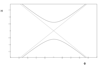
We distinguish the cases $v_0 > 0$, $v_0 = 0$ and $v_0 < 0$. The stationary points are represented graphically by the curves in the $\varphi$-$H$-plane in figure.
- Critical curves $H'[\varphi] = 0$ for quadratic potentials with $v_0
a)
b)
c)


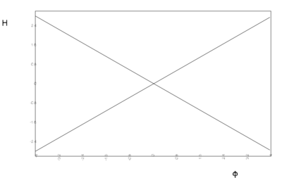
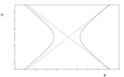
Critical curves $H'[\varphi] = 0$ for quadratic potentials with $v_0 > 0$ (a)), $v_0 = 0$ (b)) and $v_0 < 0$ (c)).
For $v_0 > 0$ there exists a stationary point for any value of $\varphi$, but the potential has a unique minimum at $\varphi = 0$, which is the only stationary point where $V' = 0$, and therefore the only end point. Indeed, once this point is reached $H$ can not decrease anymore and we have final state of de Sitter type.
For $v_0 = 0$ the critical curves become straight lines, crossing at the origin where $H = 0$ at $V = 0$. This is still a stationary point with $\ddot{\varphi} = 0$ representing a Minkoswki state, but as $V'$ is not defined there it is really to be interpreted as a limit of the previous case. There are no evolution curves flowing from the domain $H > 0$ to the domain $H < 0$.
For $v_0 < 0$ there are no stationary points in the region $\varphi^2 < 2 |v_0| /m^2$, and the solutions can cross into the domain of negative $H$ there.
Problem 12
problem id: SSC_7
Obtain actual solutions for the model of previous problem using the power series expansion \[ H[\varphi] = h_0 + h_1 \varphi + h_2 \varphi^2 + h_3 \varphi^3 + ... \] Consider the cases of $v_0 > 0$ and $v_0 < 0$.
Substitution into equation $2 H^{\prime\, 2} - 3 H^2 + V(\varphi) = 0 $ then leads to the equalities \[ 3 h_0^2 - 2 h_1^2 = v_0, \quad h_1(3h_0 - 4 h_2) = 0, \quad 4h_1(h_1 - 4 h_3) + \frac{8}{3}\, h_2 ( 3 h_0 - 4 h_2 ) = m^2, \quad ..., \] from which the solutions $H[\varphi]$ can be reconstructed (see figure below).


Problem 13
problem id: SSC_8
Estimate main contribution to total expansion factor of the Universe.
Using the results of previous problem, one can define the number of $e$-folds in some interval of time: \[ N = \int_{t_1}^{t_2} dt H = - \int_{\varphi_1}^{\varphi_2} d\varphi\, \frac{H}{2H'} = - \frac{1}{2}\, \int_{\varphi_1}^{\varphi_2} d\varphi\, \frac{h_0 + h_1 \varphi + h_2 \varphi^2 + ...}{h_1 + 2 h_2 \varphi + 3 h_3 \varphi^2 + ...}. \] This number can get sizeable contributions only in regions where the slow-roll condition is satisfied: \[ \varepsilon = - \frac{\dot{H}}{H^2} = \frac{2H^{\prime\, 2}}{H^2} < 1 \quad \Rightarrow \quad 3H^2 - V < H^2. \] Thus we simultaneously have \[ V < 3 H^2 \quad \mbox{and} \quad V > 2H^2 \quad \Leftrightarrow \quad 0 \leq \frac{V}{3} < H^2 < \frac{V}{2}. \] In most cases this holds only for a relatively narrow range of field values.
Problem 14
problem id: SSC_9_0
Explain difference between end points and turning points of the scalar field evolution.
In both cases $\dot{\varphi} = 0$, but at end points in addition $\ddot{\varphi} = 0$, which can happen only at extrema of the potential $V[\varphi]$. However, if the end point occurs at a relative maximum or saddle point of the potential, this end point will be classically unstable. Indeed, the field can remain there for an indefinite period of time, but any slight change in the initial conditions will cause it to move on to lower values of the Hubble parameter. Nevertheless, such a period of temporary slow roll of the field creates the right conditions for a period of inflation.
Problem 15
problem id: SSC_9
Show that the exponentially decaying scalar field \[ \varphi(t) = \varphi_0 e^{-\omega t} \] can give rise to unstable end points of the evolution.
The Hubble parameter and potential giving rise to this solution can be constructed following the same procedure as for the eternally oscillating field (see problem #SSC_2), with the result \[ H = h + \frac{1}{4}\, \omega \varphi^2, \quad V[\varphi] = v_0 - \frac{\mu^2}{2}\, \varphi^2 + \frac{\lambda}{4}\, \varphi^4, \] where \[ v_0 = 3 h^2, \quad \mu^2 = \omega^2 - 3 \omega h, \quad \lambda = \frac{3 \omega^2}{4}. \] Thus we obtain a quartic potential; for $\mu^2 > 0$ it has minima in which reflection symmetry is spontaneously broken. The exponential solution ends asymptotically at the unstable maximum of the potential where $\dot{\varphi} = \ddot{\varphi} = 0$. As such it represents an end point of the evolution, but a minimal change in the initial conditions for the scalar field will turn the end point into a reflection point (if it starts at lower $H$), or it will overshoot the maximum (if it starts at higher $H$). Thus the end point is unstable, but the exponential decay will still provide a good approximation to first part of the evolution of the universe for solutions $H[\varphi]$ coming close to the maximum of the potential (see figure below).

Problem 16
problem id: SSC_10
Analyze all possible final states in the model of previous problem.
The exponential scalar field leads to a behavior of the scale factor given by \[ a(t) = a_0\, e^{ht + \frac{1}{8} \varphi^2_0\, (1 - e^{-2\omega t})}. \] Thus for $h > 0$ this epoch in the evolution of the Universe ends in an asymptotic de Sitter state with Hubble constant $h$. Afterwards, the scalar field will roll further down the potential; provided $3h \leq \omega \leq 6h$ it will oscillate around the minimum until it comes to rest in another de Sitter or a Minkowski state, again depending on the value of $h$. In particular, for $\omega \geq 3h$ the model has a final de Sitter or Minkowski state in which $\dot{\varphi} = 0$ and \[ \langle \varphi^2 \rangle = \frac{\mu^2}{\lambda} = \frac{4}{3} \left(1 - \frac{3h}{\omega} \right). \] In this final state the energy density is \[ \langle V \rangle = v_0 - \frac{\mu^4}{4\lambda} = \frac{\omega}{3} ( 6h - \omega ). \]
Problem 17
problem id: SSC_11
Express initial energy density of the model of problem #SSC_9 in terms of the $e$-folding number $N$.
The energy density for the solution of problem #SSC_9 is \[ \rho_s(t) = \frac{1}{2}\, \dot{\varphi}^2 + V = 3 H^2 = 3 \left( h + \frac{1}{4}\, \omega\, \varphi_0^2\, e^{-2 \omega t} \right)^2. \] Now the solution for the scale factor \[ a(t) = a_0\, e^{ht + \frac{1}{8} \varphi^2_0\, (1 - e^{-2\omega t})}. \] shows, that before reaching the first turning point at $\varphi = 0$ the scale factor increases by an additional number of $e$-folds given by \[ N = \frac{1}{8}\, \varphi_0^2. \] Therefore the initial energy density at $t = 0$ can be written as \[ \rho_s(0) = 3 ( h + 2N \omega )^2. \] If we take this initial energy density to equal the Planck density: $\rho_s(0) = 1$, this establishes a simple relation between $h$, $\omega$ and $N$.
Problem 18
problem id: SSC_12
Estimate mass of the particles corresponding to the exponential scalar field considered in problem #SSC_9.
Taking the final energy density $\langle V \rangle$ (see problem #SSC_10) equal to the observed energy density of the Universe today: \[ \langle V \rangle = 3 H_0^2 = 1.04 \times 10^{-120} \] in Planck units, being so close to zero, one can set to an extremely good approximation $\omega = 6h$, and \[ 3 h^2 ( 1 + 12 N )^2 = 1, \quad \mu^2 = 18 h^2, \quad \lambda = 27 h^2. \] The lower limit on $N$ for inflation as derived from the CMB observations is $N \geq 60$, which requires \begin{equation} h \leq 0.8 \times 10^{-3}.\label{h_estimate} \end{equation} Now expanding $\varphi$ around its vacuum expectation value \[ \varphi = \frac{\mu}{\sqrt{\lambda}} + \chi, \] the potential becomes \[ V = \frac{1}{2}\, m_{\chi}^2 \chi^2 + \frac{\alpha}{3}\, m_{\chi} \chi^3 + \frac{\lambda}{4}\, \chi^4, \] where \[ m_{\chi} = 6h, \quad \alpha = 9h , \quad \lambda = 27 h^2. \] According to the estimate (\ref{h_estimate}) the upper limits on these parameters are \[ m_{\chi} = 0.48 \times 10^{-2}, \quad \alpha = 0.72 \times 10^{-2}\approx1/137, \quad \lambda = 0.17 \times 10^{-4}. \] Converting to particle physics units, the upper limit on the mass is $m_{\chi} \leq 1.2 \times 10^{-16}$ GeV. This suggests that the inflaton could be associated with a GUT scalar of Brout-Englert-Higgs type.
Problem 19
problem id: SSC_13
Calculate the deceleration parameter for flat Universe filled with the scalar field in form of quintessence.
There are several ways to obtain the result:
1) \[q=-\frac{\ddot a }{aH^2};\quad \frac{\ddot a}{a}=-\frac16(\rho+3p);\quad H^2=\frac13\rho;\]
\[q=\frac{\dot\varphi^2-V}{\frac{\dot\varphi^2}2+V};\]
2) \[q=\frac12\Omega_{tot}+\frac32\sum\limits_iw_i\Omega_i.\] For a flat single-component Universe one obtains
\[q=\frac12+\frac32w=\frac12+\frac32\frac{\dot\varphi^2-2V}{\dot\varphi^2+2V}=\frac{\dot\varphi^2-V}{\frac{\dot\varphi^2}2+V};\]
3) \[q=\frac{d}{dt}\frac 1 H-1=-\frac{\dot H}{H^2}-1=\frac{3H^2-V}{H^2}-1=\frac{2H^2-V}{H^2}=\frac{\dot\varphi^2-V}{\frac{\dot\varphi^2}2+V}\]
Problem 20
problem id: SSC_14_
When considering dynamics of scalar field $\varphi$ in flat Universe, let us define a function $f(\varphi)$ so that $\dot\varphi=\sqrt{f(\varphi)}$. Obtain the equation describing evolution of the function $f(\varphi)$. (T. Harko, F. Lobo and M. K. Mak, Arbitrary scalar field and quintessence cosmological models, arXiv: 1310.7167)
By substituting the Hubble function \[H^2=\frac13\left(\frac12\dot\varphi^2+V(\varphi)\right)\] into the Klein-Gordon equation we obtain \[\ddot\varphi+\sqrt3\sqrt{\frac12\dot\varphi^2+V(\varphi)}\dot\varphi + \frac{dV}{d\varphi}=0\] Introducing $\dot\varphi=\sqrt{f(\varphi)}$ and changing the independent variable from $t$ to $\varphi$, transform last equation into \[\frac12\frac{df(\varphi)}{d\varphi}+\sqrt3\sqrt{\frac12f(\varphi+V(\varphi)}\sqrt{f(\varphi)}+\frac{dV}{d\varphi}=0.\]
Exact Solutions for the Single Scalar Cosmology
after Harko (arXiv:1310.7167v4)
Problem 21
problem id: ES_0
Rewrite the equations of the single scalar cosmology \begin{equation} 3H^{2} =\rho _{\phi }=\frac{\dot{\phi}^{2}}{2}+V\left( \phi \right) , \label{H} \end{equation} \begin{equation} 2\dot{H}+3H^{2}=-p_{\phi }=-\frac{\dot{\phi}^{2}}{2}+V\left( \phi \right), \label{H1} \end{equation} \begin{equation} \ddot{\phi}+3H\dot{\phi}+V^{\prime }\left( \phi \right) = 0, \label{phi} \end{equation} in terms of the parameter $G(\phi)$ introduced as \[\dot\phi^2=2V(\phi)\sinh^2 G(\phi).\]
\begin{equation} \frac{dG}{d\phi }+\frac{1}{2V}\frac{dV}{d\phi }\coth G+\sqrt{\frac{3}{2}}=0. \label{fin} \end{equation}
Problem 22
problem id: ES_1
Obtain equation to determine the parameter $G$ as function of time.
\begin{equation} \frac{dG}{dt}=-\sqrt{2V\left( \phi \right) }\sinh G\left[ \sqrt{\frac{3}{2}}+% \frac{1}{2V\left( \phi \right) }\frac{dV}{d\phi }\coth G\right] . \label{time} \end{equation}
Problem 23
problem id: ES_2
Obtain equation to determine the parameter $G$ as function of scale factor.
\begin{equation} \frac{1}{a}\frac{da}{dG}=-\frac{1}{\sqrt{6}}\frac{\coth G}{\sqrt{\frac{3}{2}}% +\frac{1}{2V}\frac{dV}{d\phi }\coth G}. \end{equation}
Problem 24
problem id: ES_3
Obtain the deceleration parameter $q$ in terms of the parameter $G$.
\begin{equation} q(\phi )=3\tanh ^{2}G(\phi )-1. \label{bb} \end{equation}
Problem 25
problem id: ES_4
Obtain solution of the equation (\ref{fin}) with \begin{equation} V=V_{0}\exp \left( \sqrt{6}\alpha _{0}\phi \right). \label{pp} \end{equation} in the case $\alpha _0\neq \pm 1$.
\begin{equation} \sqrt{\frac{3}{2}}\left[ \phi (G)-\phi _{0}\right] =\frac{G-\alpha _{0}\ln \left| \sinh G+\alpha _{0}\cosh G\right| }{\alpha _{0}^{2}-1}\,, \label{expphi} \end{equation} \begin{equation} t(G)-t_{0}=-\frac{1}{\sqrt{3V_{0}}}\int {\frac{dG}{e^{\sqrt{3/2}\alpha _{0}\phi }\left( \sinh G+\alpha _{0}\cosh G\right) }}. \label{exp1b} \end{equation} \begin{equation} a(G)=a_{0}e^{\left[ \alpha _{0}/3\left( 1-\alpha _{0}^{2}\right) \right] G}\left( \sinh G+\alpha _{0}\cosh G\right) ^{1/3\left( \alpha _{0}^{2}-1\right) }. \end{equation}


Problem 26
problem id: ES_5
Obtain explicit solution of the problem #ES_4 in the case $\alpha _{0}=\pm \sqrt{2}$.
\begin{equation} t_{\pm }(G)-t_{0}^{\pm }=-\frac{e^{\mp \left( \sqrt{2}G+\sqrt{3}\phi _{0}\right) }}{\sqrt{3V_{0}}}\left[ 3\cosh G\pm 2\sqrt{2}\sinh G\right] . \end{equation}
Problem 27
problem id: ES_6
Obtain explicit solution of the problem #ES_4 in the case $\alpha _{0}=\pm \sqrt{3/2}$.
\begin{eqnarray} t_{\pm }(G)-t_{0}^{\pm }=\pm \frac{1}{24\sqrt{V_{0}}}\mathbf{e}^{\mp \left( \sqrt{6}G+\frac{3\phi _{0}}{2}\right) } \times \nonumber\\ \times \left[ \sqrt{2}+ 27\sqrt{2}\cosh (2G)\pm 22\sqrt{3}\sinh (2G)\right] \end{eqnarray}
Problem 28
problem id: ES_7
Obtain explicit solution of the problem #ES_4 in the case $\alpha _{0}=\pm 2/\sqrt{3}$.
\begin{eqnarray} t_{\pm }(G)-t_{0}^{\pm } =\frac{1}{396\sqrt{3V_{0}}}e^{\mp \left( 2\sqrt{3} G+\sqrt{2}\phi _{0}\right) }\Big\{ 45\cosh G\nonumber\\ +1067\cosh (3G)\pm 8\sqrt{3} \left[ 3\sinh G+77\sinh (3G)\right] \Big\} . \end{eqnarray}
Problem 29
problem id: ES_8
Obtain a particular solution of the problem #ES_4 in the case $G(\phi)=G_{0}=\mathrm{constant}$.
\begin{equation} G_{0}=\mathrm{arccoth}\left( -\frac{1}{\alpha _{0}}\right) =\frac{1}{2}\ln \left| \frac{1-\alpha _{0}}{1+\alpha _{0}}\right| , 0<|\alpha_0|<1. \end{equation} \begin{equation} a(t)=a_{0}\left[ \pm \sqrt{3V_{0}}\alpha _{0}\sinh \left( G_{0}\right) \left( t_0-t\right) \right] ^{\frac{1}{3\alpha _{0}^{2}}}. \end{equation} \begin{equation} e^{-\sqrt{3/2}\alpha _{0}\phi(t) }=\pm \sqrt{3V_{0}}\alpha _{0}\sinh \left( G_{0}\right) \left( t_{0}-t\right) , \end{equation} where $t_{0}$ is an arbitrary integration constant. \begin{eqnarray}\label{potsimpl} V(t)&=&\frac{V_{0}}{3V_{0}\alpha _{0}^{2}\sinh ^{2}\left( G_{0}\right) }\frac{1 }{\left( t-t_{0}\right) ^{2}}\nonumber\\ &=&\left( \frac{1-\alpha _{0}^{2}}{3\alpha _{0}^{4}}\right) \frac{1}{\left( t-t_{0}\right) ^{2}}=\frac{V_{0}}{\left( t-t_{0}\right) ^{2}}, \end{eqnarray} with the constants $V_{0}$, $\alpha _{0}$ and $ G_{0}$ satisfying the consistency condition \begin{equation} 3V_{0}\alpha _{0}^{2}\sinh ^{2}\left(G_{0}\right)=1. \end{equation}
Problem 30
problem id: ES_9
Obtain solution of the problem #ES_4 in the case $\alpha _0= \pm 1$.
\begin{equation} \sqrt{24}\left[ \phi (G)-\phi _{0}^{+}\right] =-e^{-2G}-2G, \qquad \alpha _{0}=+1, \end{equation} and \begin{equation} \sqrt{24}\left[ \phi (G)-\phi _{0}^{-}\right] =\ln \left| \frac{\coth G-1}{ \coth G+1}\right| +e^{2G}-1, \quad \alpha _{0}=-1, \end{equation} respectively, where $\phi _{0}^{+}$ and $\phi _{0}^{-}$ are arbitrary constants of integration. \begin{equation} t(G)-t_{0}^{+}=-\frac{1}{\sqrt{3V_{0}}}\int \frac{e^{-\sqrt{3/2}\phi }}{ \sinh G+\cosh G}dG, \qquad \alpha _{0}=+1, \end{equation} and \begin{equation} t(G)-t_{0}^{-}=-\frac{1}{\sqrt{3V_{0}}}\int \frac{e^{\sqrt{3/2}\phi }}{\sinh G-\cosh G}dG, \qquad \alpha _{0}=-1, \end{equation} respectively, where $t_{0}^{+}$ and $t_{0}^{-}$ are arbitrary constants of integration. The explicit dependence of the physical time on the parameter $G$ reads \begin{eqnarray} t(G)-t_{0}^{+}&=&-\frac{e^{-\sqrt{3/2}\phi _{0}^{+}}}{\sqrt{3V_{0}}} \int \frac{\exp \left[ (1/4)\left( e^{-2G}+2G\right) \right] }{\sinh G+\cosh G}dG, \nonumber\\ && \alpha _{0}=+1, \end{eqnarray} and \begin{eqnarray} &&t(G)-t_{0}^{-}=-\frac{e^{\sqrt{3/2}\phi _{0}^{-}}}{\sqrt{3V_{0}}}\times \nonumber\\ &&\int \frac{ \left[ (\coth G-1)/(\coth G+1)\right] ^{1/4}\exp \left[ (1/4)\left( e^{2G}-1\right) \right] }{\sinh G-\cosh G}dG, \nonumber\\ &&\alpha _{0}=-1, \end{eqnarray} respectively. The parametric dependence of the scale factor is given by \begin{equation} a(G)=a_{0}^{+}\exp \left[ \frac{1}{12}\left( 2G-e^{-2G}\right) \right] , \qquad \alpha _{0}=+1, \end{equation} and \begin{equation} a(G)=a_{0}^{-}\exp \left[ \frac{1}{12}\left( e^{2G}+2G\right) \right] , \qquad \alpha_{0}=-1, \end{equation} respectively, where $a_{0}^{+}$ and $a_{0}^{-}$ are arbitrary constants of integration.
Problem 31
problem id: ES_10
Obtain solution of the equation (\ref{fin}) with \begin{equation} \frac{1}{2V}\frac{dV}{d\phi }=\sqrt{\frac{3}{2}}\;\alpha _{1}\,\tanh G, \end{equation} where $\alpha _{1}$ is an arbitrary constant.
With this choice, the evolution equation (\ref{fin}) takes the simple form \begin{equation} \frac{dG}{d\phi }=\sqrt{\frac{3}{2}}\left( 1+\alpha _{1}\right) , \end{equation} with the general solution given by \begin{equation} G\left( \phi \right) =\sqrt{\frac{3}{2}}\left( 1+\alpha _{1}\right) \left( \phi -\phi _{0}\right) , \end{equation} where $\phi _{0}$ is an arbitrary constant of integration. \begin{equation} V\left( \phi \right) =V_{0}\cosh ^{\frac{2\alpha _{1}}{1+\alpha _{1}}}\left[ \sqrt{\frac{3}{2}}\left( 1+\alpha _{1}\right) \left( \phi -\phi _{0}\right) \right] . \label{kkk} \end{equation} \begin{equation} t-t_{0}=\frac{1}{\sqrt{2V_{0}}} \int \frac{d\phi }{\cosh ^{\frac{\alpha _1}{ 1+\alpha _1}}\left[ \sqrt{\frac{3}{2}}\left( 1+\alpha _1\right) \left( \phi -\phi _{0}\right) \right] \sinh \left[ \sqrt{\frac{3}{2}}\left( 1+\alpha _1 \right) \left( \phi -\phi _{0}\right) \right] }. \end{equation} \begin{equation} a=a_{0}\sinh ^{\frac{1}{3\left( 1+\alpha _1\right) }}\left[ \sqrt{\frac{3}{2} }\left( 1+\alpha _1\right) \left( \phi -\phi _{0}\right) \right] , \end{equation} \begin{equation} q=3\tanh ^{2}\left[ \sqrt{\frac{3}{2}}\left( 1+\alpha _1\right) \left( \phi -\phi _{0}\right) \right] -1. \end{equation}


Problem 32
problem id: ES_11
Obtain solution of the equation (\ref{fin}) for the case \begin{equation} G=\mathrm{arccoth}\left( \sqrt{\frac{3}{2}}\frac{\phi }{\alpha _{2}}\right) ,\qquad \alpha _{2}=\mathrm{constant}. \end{equation}
\begin{equation} V\left( \phi \right) =V_{0}\left( \frac{\phi }{\alpha _{2}}\right) ^{-2\left( \alpha _{2}+1\right) }\left[ \frac{3}{2}\left( \frac{\phi }{ \alpha _{2}}\right) ^{2}-1\right] , \label{mmm} \end{equation} where $V_{0}$ is an arbitrary constant of integration. \begin{equation} \frac{\phi (t)}{\alpha _{2}}=\left[ \frac{\sqrt{2V_{0}}\left( \alpha _{2}+2\right) }{\alpha _{2}}\right] ^{\frac{1}{\alpha _{2}+2}}\left( t-t_{0}\right) ^{\frac{1}{\alpha _{2}+2}}. \end{equation} \begin{equation} a=a_{0}\exp \left( \frac{\phi ^{2}}{4\alpha _{2}}\right) = a_0\exp \left\{ \frac{1}{4\alpha _{2}}\left[ \frac{\left( \alpha _{2}+2\right) \sqrt{2V_{0}} }{\alpha _{2}}\right] ^{\frac{2}{\alpha _{2}+2}}\left( t-t_{0}\right) ^{ \frac{2}{\alpha _{2}+2}}\right\} , \end{equation} with $a_{0}$ an arbitrary constant of integration. The deceleration parameter is given by \begin{equation} q=2\left( \frac{\phi }{\alpha _{2}}\right) ^{-2}-1= 2\left[ \frac{\sqrt{2V_{0} }\left( \alpha _{2}+2\right) }{\alpha _{2}}\right] ^{-\frac{2}{\alpha _{2}+2} }\left( t-t_{0}\right) ^{-\frac{2}{\alpha _{2}+2}}-1. \end{equation}
Problem 33
problem id: ES_12
Rewrite the equation (\ref{fin}) in form of the two linear differential equations for the variable $w=e^{-G}$.
\begin{equation} \frac{dw}{d\phi }+\left[ \alpha _{3}+S\left( \phi \right) \right] w=M\left( \phi \right) , \label{n2} \end{equation} and \begin{equation} \frac{dw^{3}}{d\phi }+3\left[ \alpha _{3}-S\left( \phi \right) \right] w^{3}=3M\left( \phi \right) , \label{n3} \end{equation} where $M\left( \phi \right)$ is a new separation function, $S\left( \phi \right) =-d\ln \left| \sqrt{V}\right| /d\phi $ and $\alpha _{3}=-\sqrt{3/2}$.
Problem 34
problem id: ES_13
Obtain a consistency integral relation between the separation function $M(\phi )$ and the self-interaction potential $V(\phi )$, corresponding to the equations for the variable $w$, obtained in the previous problem.
Equation~(\ref{n2}) can be integrated to provide \begin{equation} w=\sqrt{V}e^{-\alpha _{3}\phi }\left[ C_{0}+\int \frac{M\left( \phi \right) e^{\alpha _{3}\phi }}{\sqrt{V}}d\phi \right] , \label{n4} \end{equation} where $C_{0}$ is an arbitrary constant of integration. Equation~(\ref{n3}) can be integrated to give \begin{equation} w=\frac{e^{-\alpha _{3}\phi }}{\sqrt{V}}\left[ C_{1}+3\int M\left( \phi \right) V^{3/2}e^{3\alpha _{3}\phi }d\phi \right] ^{1/3}, \label{n5} \end{equation} where $C_{1}$ is an arbitrary constant of integration. Then the consistency relation reads \begin{equation} C_{1}+3\int M\left( \phi \right) V^{3/2}e^{3\alpha _{3}\phi }d\phi =V^{3} \left[ C_{0}+\int \frac{M\left( \phi \right) e^{\alpha _{3}\phi }}{\sqrt{V}} d\phi \right] ^{3}. \label{n7} \end{equation}
Problem 35
problem id: ES_14
Obtain exact solution of the equation (\ref{fin}) in the case $M\left( \phi \right) =\sqrt{V}$.
The consistency relation (\ref{n7}) now reads \begin{equation} C_{1}+3\int V^{2}e^{3\alpha _{3}\phi }d\phi =V^{3}A\left( \phi \right) , \label{n8} \end{equation} where we have denoted $A(\phi )=\left( C_{0}+e^{\alpha _{3}\phi }/\alpha _{3}\right) ^{3}$. In order to solve the integral Eq.~(\ref{n8}), we rewrite it as a linear first order differential equation for $V\left( \phi \right) $ \begin{equation} \frac{dV}{d\phi }+\left[ \frac{d}{d\phi }\left( \ln A^{1/3}\right) \right] V= \frac{e^{3\alpha _{3}\phi }}{A\left( \phi \right) }, \label{n9} \end{equation} with the general solution given by \begin{equation} V(\phi )=A^{-1/3}\left( \phi \right) \left[ C_{2}+\int e^{3\alpha _{3}\phi }A^{-2/3}\left( \phi \right) d\phi \right] , \label{nn} \end{equation} where $C_{2}$ is an arbitrary constant of integration. Now by inserting $ A\left( \phi \right) $ into Eq.~(\ref{nn}) yields the expression of the scalar field potential as \begin{equation} V(\phi )=\frac{\alpha _{3}^{2}\left\{ e^{3\alpha _{3}\phi }+2C_{0}\alpha _{3}e^{2\alpha _{3}\phi }-C_{0}^{3}\alpha _{3}^{3}+\left( C_{0}\alpha +e^{\alpha _{3}\phi }\right) ^{2}\left[ \frac{C_{2}}{\alpha _{3}} -2C_{0}\alpha _{3}\ln \left| C_{0}\alpha _{3}+e^{\alpha _{3}\phi }\right| \right] \right\} }{\left( C_{0}\alpha _{3}+e^{\alpha _{3}\phi }\right) ^{3}}. \label{pot1} \end{equation} Therefore the general solution of Eq.~(\ref{fin}) is given by \begin{equation} G=\mathrm{arccoth}\left( \frac{ 1+w^{2}} { 1-w^{2}} \right) =\ln \left| \frac{1}{w}\right| , \end{equation} where \begin{equation} w(\phi )=\sqrt{V(\phi )} e^{-\alpha _{3}\phi }\left( C_{0}+\frac{e^{\alpha _{3}\phi }}{\alpha _{3}}\right) . \end{equation}
Problem 36
problem id: ES_15
Obtain exact solution of the equation (\ref{fin}) in the case $M\left( \phi \right) =V^{-3/2}$.
The consistency relation (\ref{n7}) now reads \begin{equation} C_{0}+\int \frac{e^{\alpha _{3}\phi }}{V^{2}}d\phi =\frac{\left( C_{1}+\frac{ 1}{\alpha _{3}}e^{3\alpha _{3}\phi }\right) ^{1/3}}{V}. \label{b1} \end{equation} In order to solve Eq.~(\ref{b1}), we rewrite it as a linear first order differential equation for $V\left( \phi \right) $ \begin{equation} \frac{dV}{d\phi }+\left[ \frac{d}{d\phi }\ln \left| \frac{1}{\left( C_{1}+ \frac{1}{\alpha _{3}}e^{3\alpha _{3}\phi }\right) ^{1/3}}\right| \right] V =-\frac{e^{\alpha _{3}\phi }}{\left( C_{1}+\frac{1}{\alpha _{3}}e^{3\alpha _{3}\phi }\right) ^{1/3}}. \label{b2} \end{equation} Equation~(\ref{b2}) can be easily integrated, and yields the following solution \begin{equation} V\left( \phi \right) =\left( C_{1}+\frac{1}{\alpha _{3}}e^{3\alpha _{3}\phi }\right) ^{1/3} \times \left[ C_{3}-\int \frac{e^{\alpha _{3}\phi }}{\left( C_{1}+ \frac{1}{\alpha _{3}}e^{3\alpha _{3}\phi }\right) ^{2/3}}d\phi \right] . \label{pot2} \end{equation} where $C_{3}$ is an arbitrary constant of integration. Therefore the general solution of Eq.~(\ref{fin}) is given by \begin{equation} G=\mathrm{arccoth}\left( \frac{ 1+w^{2}}{1-w^{2}} \right) =\ln \left| \frac{1}{w}\right| , \end{equation} where \begin{equation} w(\phi )=\left[ \frac{e^{-\alpha _{3}\phi }}{\sqrt{V(\phi )}}\right] \left( C_{1}+\frac{e^{3\alpha _{3}\phi }}{\alpha _{3}}\right) ^{1/3}. \end{equation}