New problems
NEW Problems in Dark Energy Category
The discovery of the Higgs particle has confirmed that scalar fields play a fundamental role in subatomic physics. Therefore they must also have been present in the early Universe and played a part in its development. About scalar fields on present cosmological scales nothing is known, but in view of the observational evidence for accelerated expansion it is quite well possible that they take part in shaping our Universe now and in the future. In this section we consider the evolution of a flat, isotropic and homogeneous Universe in the presence of a single cosmic scalar field. Neglecting ordinary matter and radiation, the evolution of such a Universe is described by two degrees of freedom, the homogeneous scalar field $\varphi(t)$ and the scale factor of the Universe $a(t)$. The relevant evolution equations are the Friedmann and Klein-Gordon equations, reading (in the units in which $c = \hbar = 8 \pi G = 1$) \[ \frac{1}{2}\, \dot{\varphi}^2 + V = 3 H^2, \quad \ddot{\varphi} + 3 H \dot{\varphi} + V' = 0, \] where $V[\varphi]$ is the potential of the scalar fields, and $H = \dot{a}/a$ is the Hubble parameter. Furthermore, an overdot denotes a derivative w.r.t.\ time, whilst a prime denotes a derivative w.r.t.\ the scalar field $\varphi$.
Problem 1
problem id: SSC_0
Show that the Hubble parameter cannot increase with time in the single scalar cosmology.
Let the scalar field $\varphi(t)$ is a single-valued function of time, then it is possible to reparametrize the Hubble parameter in terms of $\varphi$: \[ H(t) = H[\varphi(t)]. \] Taking time derivatives in the Friedman equation \[ \frac{1}{2}\, \dot{\varphi}^2 + V = 3 H^2, \] one arrives at the results: \[ \dot{\varphi} ( \ddot{\varphi} + V' ) = 6 H \dot{H},\quad \dot{H} \equiv H' \dot{\varphi}. \] Taking into account the Klein Gordon equation \[ \ddot{\varphi} + 3 H \dot{\varphi} + V' = 0, \] it follows, that for $\dot{\varphi} \neq 0$ and $H \neq 0$ one gets \[ \dot{\varphi} = - 2 H', \quad \dot{H} = - \frac{1}{2}\, \dot{\varphi}^2 \leq 0. \] Thus the Hubble parameter is a semi-monotonically decreasing function of time.
Problem 2
problem id: SSC_1
Obtain first-order differential equation for the Hubble parameter $H$ as function of $\varphi$ and find its stationary points.
Replacing the time derivatives in the Friedmann equation using the results of the previous problem, one finds \[ 2 H^{\prime\, 2} - 3 H^2 + V(\varphi) = 0. \] There are two kinds of stationary points; a point where $\dot{\varphi} = H' = 0$ is an end point of the evolution if \[ \ddot{\varphi} = 4 H' H'' = 0, \] which happens if $H''$ is finite. In contrast, if \[ \ddot{\varphi} = 4 H' H'' \neq 0, \] $H''$ necessarily diverges in such a way as to make $\ddot{\varphi}$ finite: $H'' \propto 1/H'$.
Problem 3
problem id: SSC_2
Consider eternally oscillating scalar field of the form $\varphi(t) = \varphi_0 \cos \omega t$ and analyze stationary points in such a model.
For such a scalar field to exist it is required that \[ H' = - \frac{1}{2}\, \dot{\varphi} = \frac{\omega \varphi_0}{2} \sin \omega t = \frac{\omega}{2} \sqrt{\varphi_0^2 - \varphi^2}. \] There are infinitely many stationary points \[ \omega t_n = n \pi, \quad \varphi(t_n) = (-1)^n \varphi_0, \] where $H' = 0$. Now \[ H'' = - \frac{1}{2} \frac{\omega \varphi}{\sqrt{\varphi_0^2 - \varphi^2}}, \] and therefore $H''$ diverges at all stationary points $t_n$, but in such a way that \[ 4 H' H'' = - \omega^2 \varphi = \ddot{\varphi}. \] Then all stationary points in the considered model are turning points.
Problem 4
problem id: SSC_3
Obtain explicit solution for the Hubble parameter in the model considered in the previous problem.
\begin{align} H & = H_0 - \frac{1}{4} \omega \varphi_0^2 \arccos \left( \frac{\varphi}{\varphi_0} \right) +\frac{1}{4} \omega \varphi \sqrt{\varphi_0^2 - \varphi^2} \\ & = H_0 - \frac{1}{4} \omega^2 \varphi_0^2 t + \frac{1}{8} \omega \varphi_0^2 \sin 2 \omega t. \end{align}
Problem 5
problem id: SSC_4
Obtain explicit time dependence for the scale factor in the model of problem #SSC_2.
The corresponding solution for the scale factor is \[ a(t) = a(0) \exp\left\{H_0 t - \frac{1}{8} \omega^2 \varphi_0^2 t^2 + \frac{1}{16} \left( 1 - \cos 2 \omega t \right)\right\}. \] which is a gaussian, slightly modulated by an oscillating function of time (see figure).

Problem 6
problem id: SSC_5
Reconstruct the scalar field potential $V(\varphi)$ needed to generate the model of problem #SSC_2.
The potential giving rise to this behavior reads \begin{align} V & = 3 H^2 - 2 H^{\prime\, 2} \\ & = 3 \left( H_0 - \frac{1}{4}\, \omega \varphi_0^2 \arccos \left( \frac{\varphi}{\varphi_0} \right) + \frac{1}{4} \omega \varphi \sqrt{ \varphi_0^2 - \varphi^2} \right)^2 - \frac{\omega^2}{2} \left( \varphi_0^2 - \varphi^2 \right). \end{align} Observe, that this potential keeps track of the number of oscillations the scalar field has performed through the arccos-function, so ultimately $V$ increases indefinitely as a function of time, whilst the volume of a representative domain of space decreases rapidly.
Problem 7
problem id: SSC_6_00
Describe possible final states for the Universe governed by a single scalar field at large times.
If $H$ becomes negative then the Universe inevitably collapses.If $H$ never becomes negative, it must tend to a vanishing or positive final minimum, which can be reached either in finite or infinite time. The universe then ends up in a Minkowski or in a de Sitter state. These conclusions are a consequence of the non-positivity of $\dot{H}$ (see problem #SSC_0, which implies that a negative $H$ can never return to larger values at later times.
Problem 8
problem id: SSC_6_0
Formulate conditions for existence of end points of evolution in terms of the potential $V(\varphi)$.
In order to establish the existence of end points or asymptotic end points of evolution at non-negative values of $H$, we first consider the locus of all stationary points, defined by \[ \dot{\varphi} = - 2 H' = 0 \quad \Rightarrow \quad V = 3 H^2 \geq 0 . \] It follows that stationary points can occur only in the region of positive or vanishing potential. In particular this holds for end points, which therefore do not occur in a region of negative potential. Moreover, it is clear that a Minkowski final state occurs only at a stationary point where $V = 0$, whereas all stationary points with $V > 0$ correspond to de Sitter states. To correspond to an end point of the evolution, $H''$ must be finite at these stationary points to guarantee that $\ddot{\varphi} = 0$ as well. From the results of the problem \ref{SSC_1} it follows that \[ V' = 2 H' (3 H - 2 H''), \] and therefore $V' = 0$ if $H' = 0$ and $H$ and $H''$ are finite. As a result end points of the evolution necessarily occur at an extremum of $V$, but only if $V \geq 0$ there.
Problem 9
problem id: SSC_6_1
Consider a single scalar cosmology described by the quadratic potential \[ V = v_0 + \frac{m^2}{2}\, \varphi^2. \] Describe all possible stationary points and final states of the Universe in this model.
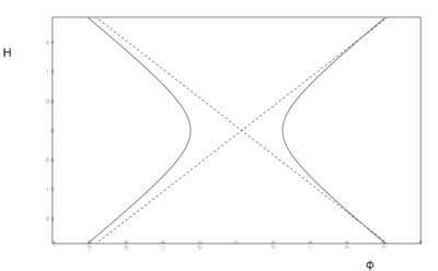
We distinguish the cases $v_0 > 0$, $v_0 = 0$ and $v_0 < 0$. The stationary points are represented graphically by the curves in the $\varphi$-$H$-plane in figure.
- Critical curves $H'[\varphi] = 0$ for quadratic potentials with $v_0
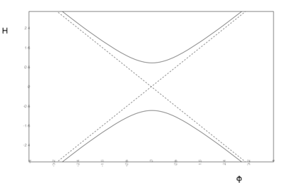


For $v_0 > 0$ there exists a stationary point for any value of $\varphi$, but the potential has a unique
minimum at $\varphi = 0$, which is the only stationary point where $V' = 0$, and therefore the only end point.
Indeed, once this point is reached $H$ can not decrease anymore and we have final state of de
Sitter type.
For $v_0 = 0$ the critical curves become straight lines, crossing at the origin where $H = 0$ at $V = 0$. This is still a stationary point with $\ddot{\varphi} = 0$ representing a Minkoswki state, but as $V'$ is not defined there it is really to be interpreted as a limit of the previous case. There are no evolution curves flowing from the domain $H > 0$ to the domain $H < 0$.
For $v_0 < 0$ there are no stationary points in the region $\varphi^2 < 2 |v_0| /m^2$, and the solutions can cross into the domain of negative $H$ there.
Problem 10
problem id:
Problem
problem id:
Problem
problem id:
Problem
problem id:
Problem
problem id:
Problem
problem id:
Problem
problem id:
Problem
problem id:
Problem
problem id:
Problem
problem id:
Problem
problem id:
Problem
problem id:
Problem
problem id:
Problem
problem id:
Problem
problem id:
Problem
problem id:
Problem
problem id:
Problem
problem id:
Problem
problem id:
Problem
problem id:
Problem
problem id:
Problem
problem id:
Problem
problem id:
Problem
problem id:
Problem
problem id:
Problem
problem id:
Problem
problem id:
Problem
problem id:
Problem
problem id:
Problem
problem id:
Problem
problem id:
Problem
problem id:
Problem
problem id:
Problem
problem id:
Problem
problem id:
Problem
problem id:
Problem
problem id:
Problem
problem id:
Problem
problem id:
Problem
problem id:
Problem
problem id:
Problem
problem id:
Problem
problem id:
Problem
problem id:
Problem
problem id:
Problem
problem id:
Problem
problem id:
Problem
problem id:
Problem
problem id:
Problem
problem id:
Problem
problem id:
Problem
problem id:
Problem
problem id:
Problem
problem id:
Problem
problem id:
Problem
problem id:
Problem
problem id:
Problem
problem id:
Problem
problem id:
Problem
problem id:
Problem
problem id:
Problem
problem id:
Problem
problem id:
Problem
problem id:
Problem
problem id:
Problem
problem id:
Problem
problem id:
Problem
problem id:
Problem
problem id:
Problem
problem id:
Problem
problem id:
Problem
problem id:
Problem
problem id:
Problem
problem id:
Problem
problem id:
Problem
problem id:
Problem
problem id:
Problem
problem id:
Problem
problem id:
Problem
problem id:
Problem
problem id:
Problem
problem id: