Difference between revisions of "New problems"
(→Problem 1) |
(→Problem 7) |
||
| Line 1,558: | Line 1,558: | ||
The most commonly used distance is the luminosity distance, and it is related to the distance modulus in the following way: | The most commonly used distance is the luminosity distance, and it is related to the distance modulus in the following way: | ||
\[\mu_D=5\log_10[d_L/(10\ pc)]=5\log_10[d_L/(1\ Mpc)]+25.\] | \[\mu_D=5\log_10[d_L/(10\ pc)]=5\log_10[d_L/(1\ Mpc)]+25.\] | ||
| − | + | However, alternative distances are also used (for a variety of mathematical purposes): | |
<br/>1) The "photon flux distance": \[d_F=\frac{d_L}{(1+z)^{1/2}}.\] | <br/>1) The "photon flux distance": \[d_F=\frac{d_L}{(1+z)^{1/2}}.\] | ||
<br/>2) The "photon count distance": \[d_P=\frac{d_L}{(1+z)}.\] | <br/>2) The "photon count distance": \[d_P=\frac{d_L}{(1+z)}.\] | ||
| Line 1,564: | Line 1,564: | ||
<br/>4) The "angular diameter distance": \[d_A=\frac{d_L}{(1+z)^{2}}.\] | <br/>4) The "angular diameter distance": \[d_A=\frac{d_L}{(1+z)^{2}}.\] | ||
| − | Obtain the Hubble law for these distances (in terms of $z$-redshift, up to the second power by z): | + | Obtain the Hubble law for these distances (in terms of $z$-redshift, up to the second power by z) |
| − | \begin{align} | + | |
| + | <div class="NavFrame collapsed"> | ||
| + | <div class="NavHead">solution</div> | ||
| + | <div style="width:100%;" class="NavContent"> | ||
| + | <p style="text-align: left;">\begin{align} | ||
\nonumber d_F(z) & =d_H z\left\{1-\frac12q_0z+O(z^2)\right\}.\\ | \nonumber d_F(z) & =d_H z\left\{1-\frac12q_0z+O(z^2)\right\}.\\ | ||
\nonumber d_P(z) & =d_H z\left\{1-\frac12(1+q_0)z+O(z^2)\right\}.\\ | \nonumber d_P(z) & =d_H z\left\{1-\frac12(1+q_0)z+O(z^2)\right\}.\\ | ||
\nonumber d_Q(z) & =d_H z\left\{1-\frac12(2+q_0)z+O(z^2)\right\}.\\ | \nonumber d_Q(z) & =d_H z\left\{1-\frac12(2+q_0)z+O(z^2)\right\}.\\ | ||
\nonumber d_A(z) & =d_H z\left\{1-\frac12(3+q_0)z+O(z^2)\right\}. | \nonumber d_A(z) & =d_H z\left\{1-\frac12(3+q_0)z+O(z^2)\right\}. | ||
| − | \end{align} | + | \end{align}</p> |
| − | + | ||
| − | + | ||
| − | + | ||
| − | + | ||
</div> | </div> | ||
| − | </div | + | </div></div> |
<div id=""></div> | <div id=""></div> | ||
<div style="border: 1px solid #AAA; padding:5px;"> | <div style="border: 1px solid #AAA; padding:5px;"> | ||
| + | |||
=== Problem 8 === | === Problem 8 === | ||
<p style= "color: #999;font-size: 11px">problem id: </p> | <p style= "color: #999;font-size: 11px">problem id: </p> | ||
Revision as of 02:02, 1 April 2014
Contents
- 1 NEW Problems in Cosmo warm-up Category
- 2 NEW Problems in Dark Energy Category
- 2.1 Single Scalar Cosmology
- 2.1.1 Problem 1
- 2.1.2 Problem 2
- 2.1.3 Problem 3
- 2.1.4 Problem 4
- 2.1.5 Problem 5
- 2.1.6 Problem 6
- 2.1.7 Problem 7
- 2.1.8 Problem 8
- 2.1.9 Problem 9
- 2.1.10 Problem 10
- 2.1.11 Problem 11
- 2.1.12 Problem 12
- 2.1.13 Problem 13
- 2.1.14 Problem 14
- 2.1.15 Problem 15
- 2.1.16 Problem 16
- 2.1.17 Problem 17
- 2.1.18 Problem 18
- 2.1.19 Problem 19
- 2.1.20 Problem 20
- 2.2 The Power-Law Cosmology
- 2.3 Hybrid Expansion Law
- 2.4 Bianchi I Model
- 2.5 Radiation dominated BI model
- 2.1 Single Scalar Cosmology
- 3 NEW problems in Dark Matter Category
- 4 Tutti Frutti
- 5 NEW problems in Observational Cosmology Category
- 6 Exact Solutions
- 7 NEW Problems in Dynamics of the Expanding Universe Category
- 7.1 Cosmography
- 7.1.1 Problem 1
- 7.1.2 Problem 2
- 7.1.3 Problem 3
- 7.1.4 Problem 4
- 7.1.5 Problem 5
- 7.1.6 Problem 6
- 7.1.7 Problem 7
- 7.1.8 Problem 8
- 7.1.9 Problem 9
- 7.1.10 Problem 10
- 7.1.11 Problem 11
- 7.1.12 Problem 12
- 7.1.13 Problem 13
- 7.1.14 Problem 14
- 7.1.15 Problem 15
- 7.1.16 Problem 16
- 7.1.17 Problem 17
- 7.1.18 Problem 18
- 7.1.19 Problem 19
- 7.1.20 Problem 20
- 7.1.21 Problem 21
- 7.1.22 Problem 22
- 7.1.23 Problem 23
- 7.1.24 Problem 24
- 7.1.25 Problem 25
- 7.1 Cosmography
NEW Problems in Cosmo warm-up Category
Play with Numbers after Sivaram
Problem 1
problem id: Siv_1
(after C.Sivaram, Dark Energy may link the numbers of Rees, arXiv: 0710.4993) Given $\Lambda$-dominated Universe, the requirement that for various large scale structures (held together by self gravity) to form a variety of length scales, their gravitational self energy density should at least match the ambient vacuum energy repulsion, as was shown to imply [16. C Sivaram, Astr. Spc. Sci, 219, 135; IJTP, 33, 2407, 1994, 17. C Sivaram, Mod. Phys. Lett., 34, 2463, 1999] a scale invariant mass-radius relationship to the form (for the various structures): \[\frac M{R^2}\approx\sqrt\Lambda\frac{c^2} G.\] This equation predicts a universality of $M/R^2$ for a large variety of structures. Check this statement for such structures as a galaxy, a globular cluster, a galaxy cluster.
For a typical spiral galaxy $M_{gal}\approx10^{12} M_\odot$, $R\approx30kpc$, for globular clusters, $M\approx10^{6} M_\odot$, $R\approx100pc$, for galaxy clusters, $M_C\approx10^{16} M_\odot$, $R_C\approx3Mpc$, so for all these structures the equation holds.
Problem 2
problem id: Siv_2
(after C.Sivaram, Scaling Relations for self-Similar Structures and the Cosmological Constant, arXiv: 0801.1218) In recent papers [13. Sivaram, C.: 1993a, Mod. Phys. Lett. 8,321.; 14. Sivaram, C.: 1993b, Astrophys. Spc. Sci. 207, 317.; 15. Sivaram, C.: 1993c, Astron. Astrophys. 275, 37.; 16. Sivaram, C.: 1994a, Astrophysics. Spc. Sci., 215, 185.; 17. Sivaram, C.: 1994b. Astrphysics .Spc .Sci., 215,191.; 18. Sivaram, C.: 1994c. Int. J. Theor. Phys. 33, 2407.], it was pointed out that the surface gravities of a whole hierarchy of astronomical objects (i.e. globular clusters, galaxies, clusters, super clusters, GMC's etc.) are more or less given by a universal value $a_0\approx cH_0\approx 10^{-8} cm\ s^{-2}$ a o ƒ° cHo ƒ° 10-8 cms-2. Thus \[a=\frac{GM}{R^2}\approx a_0\] for all these objects, $M$ being their typical mass and $R$ their typical radius. Also interestingly enough it was also pointed out [4. Sivaram, C.: 1982, Astrophysics. Spc. Sci. 88,507.; 5. Sivaram, C.: 1982, Amer. J. Phy. 50, 279.; 6. Sivaram, C.: 1983, Amer. J. Phys. 51, 277.; 7. Sivaram, C.: 1983, Phys. Lett. 60B, 181.] that the gravitational self energy of a typical elementary particle (hadron) was shown to be \[E_G\approx\frac{Gm^3 c}{\hbar}\approx\hbar H_0\] implying the same surface gravity value for the particle \[a_h=\frac{GM}{r^2}\approx \frac{Gm^3 c}{\hbar}\times\frac c\hbar\approx cH_0\approx a_0.\] Calculate actual value of the ratio \[\frac M{R^2}\approx\sqrt\Lambda\frac{c^2} G\sim1\] for such examples as a galaxy, whole Universe, globular cluster, a GMC, a supercluster, nuclei, an electron, Solar system, planetary nebula.
\begin{tabular}{|c|c|} \hline UNIQ-MathJax12-QINU (UNIQ-MathJax13-QINU) & Object \\ \hline UNIQ-MathJax14-QINU & Galaxy \\ UNIQ-MathJax15-QINU & Universe \\ UNIQ-MathJax16-QINU & globular cluster, GMC, etc. \\ UNIQ-MathJax17-QINU & supercluster \\ UNIQ-MathJax18-QINU & nuclei \\ UNIQ-MathJax19-QINU & electron \\ UNIQ-MathJax20-QINU & Solar system, planetary nebula\\ \hline \end{tabular}
NEW Problems in Dark Energy Category
Single Scalar Cosmology
The discovery of the Higgs particle has confirmed that scalar fields play a fundamental role in subatomic physics. Therefore they must also have been present in the early Universe and played a part in its development. About scalar fields on present cosmological scales nothing is known, but in view of the observational evidence for accelerated expansion it is quite well possible that they take part in shaping our Universe now and in the future. In this section we consider the evolution of a flat, isotropic and homogeneous Universe in the presence of a single cosmic scalar field. Neglecting ordinary matter and radiation, the evolution of such a Universe is described by two degrees of freedom, the homogeneous scalar field $\varphi(t)$ and the scale factor of the Universe $a(t)$. The relevant evolution equations are the Friedmann and Klein-Gordon equations, reading (in the units in which $c = \hbar = 8 \pi G = 1$) \[ \frac{1}{2}\, \dot{\varphi}^2 + V = 3 H^2, \quad \ddot{\varphi} + 3 H \dot{\varphi} + V' = 0, \] where $V[\varphi]$ is the potential of the scalar fields, and $H = \dot{a}/a$ is the Hubble parameter. Furthermore, an overdot denotes a derivative w.r.t.\ time, whilst a prime denotes a derivative w.r.t.\ the scalar field $\varphi$.
Problem 1
problem id: SSC_0
Show that the Hubble parameter cannot increase with time in the single scalar cosmology.
Let the scalar field $\varphi(t)$ is a single-valued function of time, then it is possible to reparametrize the Hubble parameter in terms of $\varphi$: \[ H(t) = H[\varphi(t)]. \] Taking time derivatives in the Friedman equation \[ \frac{1}{2}\, \dot{\varphi}^2 + V = 3 H^2, \] one arrives at the results: \[ \dot{\varphi} ( \ddot{\varphi} + V' ) = 6 H \dot{H},\quad \dot{H} \equiv H' \dot{\varphi}. \] Taking into account the Klein Gordon equation \[ \ddot{\varphi} + 3 H \dot{\varphi} + V' = 0, \] it follows, that for $\dot{\varphi} \neq 0$ and $H \neq 0$ one gets \[ \dot{\varphi} = - 2 H', \quad \dot{H} = - \frac{1}{2}\, \dot{\varphi}^2 \leq 0. \] Thus the Hubble parameter is a semi-monotonically decreasing function of time.
Problem 2
problem id: SSC_00
Show that if the Universe is filled by a substance which satisfies the null energy condition then the Hubble parameter is a semi-monotonically decreasing function of time.
\[\dot H=-\frac12(\rho+p).\] If $\rho+p\ge0$ (null energy condition), $H$ is a semi-monotonically decreasing function of time.
Problem 3
problem id: SSC_0_1
For single-field scalar models express the scalar field potential in terms of the Hubble parameter and its derivative with respect to the scalar field.
For single-field models in which the scalar field is a single-valued function of time in some interval, it is possible to reparametrize the Hubble parameter in terms of $\varphi$: \[H(t)=H[\varphi(t)]\] Replacing the time derivatives $\dot{\varphi} = - 2 H'$ (see the problem \ref{SSC_0}) in the Friedmann equation we find \[V=3H^2-2H'^2.\] The latter expression can be used to reconstruct the potential if the evolution history $H[\varphi(t)]$ is known, or for given $V(\varphi)$ this is a first-order differential equation for $H[\varphi(t)]$.
Problem 4
problem id: SSC_1
Obtain first-order differential equation for the Hubble parameter $H$ as function of $\varphi$ and find its stationary points.
Replacing the time derivatives in the Friedmann equation using the results of the previous problem, one finds \[ 2 H^{\prime\, 2} - 3 H^2 + V(\varphi) = 0. \] There are two kinds of stationary points; a point where $\dot{\varphi} = H' = 0$ is an end point of the evolution if \[ \ddot{\varphi} = 4 H' H'' = 0, \] which happens if $H''$ is finite. In contrast, if \[ \ddot{\varphi} = 4 H' H'' \neq 0, \] $H''$ necessarily diverges in such a way as to make $\ddot{\varphi}$ finite: $H'' \propto 1/H'$.
Problem 5
problem id: SSC_2
Consider eternally oscillating scalar field of the form $\varphi(t) = \varphi_0 \cos \omega t$ and analyze stationary points in such a model.
For such a scalar field to exist it is required that \[ H' = - \frac{1}{2}\, \dot{\varphi} = \frac{\omega \varphi_0}{2} \sin \omega t = \frac{\omega}{2} \sqrt{\varphi_0^2 - \varphi^2}. \] There are infinitely many stationary points \[ \omega t_n = n \pi, \quad \varphi(t_n) = (-1)^n \varphi_0, \] where $H' = 0$. Now \[ H'' = - \frac{1}{2} \frac{\omega \varphi}{\sqrt{\varphi_0^2 - \varphi^2}}, \] and therefore $H''$ diverges at all stationary points $t_n$, but in such a way that \[ 4 H' H'' = - \omega^2 \varphi = \ddot{\varphi}. \] Then all stationary points in the considered model are turning points.
Problem 6
problem id: SSC_3
Obtain explicit solution for the Hubble parameter in the model considered in the previous problem.
\begin{align} H & = H_0 - \frac{1}{4} \omega \varphi_0^2 \arccos \left( \frac{\varphi}{\varphi_0} \right) +\frac{1}{4} \omega \varphi \sqrt{\varphi_0^2 - \varphi^2} \\ & = H_0 - \frac{1}{4} \omega^2 \varphi_0^2 t + \frac{1}{8} \omega \varphi_0^2 \sin 2 \omega t. \end{align}
Problem 7
problem id: SSC_4
Obtain explicit time dependence for the scale factor in the model of problem #SSC_2.
The corresponding solution for the scale factor is \[ a(t) = a(0) \exp\left\{H_0 t - \frac{1}{8} \omega^2 \varphi_0^2 t^2 + \frac{1}{16} \left( 1 - \cos 2 \omega t \right)\right\}. \] which is a gaussian, slightly modulated by an oscillating function of time (see figure).

Problem 8
problem id: SSC_5
Reconstruct the scalar field potential $V(\varphi)$ needed to generate the model of problem #SSC_2.
The potential giving rise to this behavior reads \begin{align} V & = 3 H^2 - 2 H^{\prime\, 2} \\ & = 3 \left( H_0 - \frac{1}{4}\, \omega \varphi_0^2 \arccos \left( \frac{\varphi}{\varphi_0} \right) + \frac{1}{4} \omega \varphi \sqrt{ \varphi_0^2 - \varphi^2} \right)^2 - \frac{\omega^2}{2} \left( \varphi_0^2 - \varphi^2 \right). \end{align} Observe, that this potential keeps track of the number of oscillations the scalar field has performed through the arccos-function, so ultimately $V$ increases indefinitely as a function of time, whilst the volume of a representative domain of space decreases rapidly.
Problem 9
problem id: SSC_6_00
Describe possible final states for the Universe governed by a single scalar field at large times.
If $H$ becomes negative then the Universe inevitably collapses.If $H$ never becomes negative, it must tend to a vanishing or positive final minimum, which can be reached either in finite or infinite time. The universe then ends up in a Minkowski or in a de Sitter state. These conclusions are a consequence of the non-positivity of $\dot{H}$ (see problem #SSC_0, which implies that a negative $H$ can never return to larger values at later times.
Problem 10
problem id: SSC_6_0
Formulate conditions for existence of end points of evolution in terms of the potential $V(\varphi)$.
In order to establish the existence of end points or asymptotic end points of evolution at non-negative values of $H$, we first consider the locus of all stationary points, defined by \[ \dot{\varphi} = - 2 H' = 0 \quad \Rightarrow \quad V = 3 H^2 \geq 0 . \] It follows that stationary points can occur only in the region of positive or vanishing potential. In particular this holds for end points, which therefore do not occur in a region of negative potential. Moreover, it is clear that a Minkowski final state occurs only at a stationary point where $V = 0$, whereas all stationary points with $V > 0$ correspond to de Sitter states. To correspond to an end point of the evolution, $H''$ must be finite at these stationary points to guarantee that $\ddot{\varphi} = 0$ as well. From the results of the problem \ref{SSC_1} it follows that \[ V' = 2 H' (3 H - 2 H''), \] and therefore $V' = 0$ if $H' = 0$ and $H$ and $H''$ are finite. As a result end points of the evolution necessarily occur at an extremum of $V$, but only if $V \geq 0$ there.
Problem 11
problem id: SSC_6_1
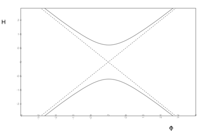
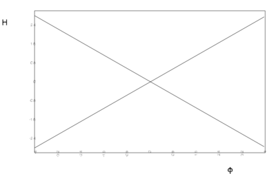
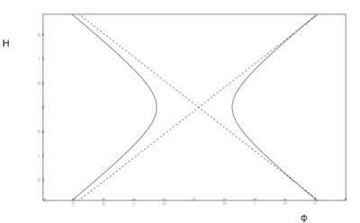
Consider a single scalar cosmology described by the quadratic potential \[ V = v_0 + \frac{m^2}{2}\, \varphi^2. \] Describe all possible stationary points and final states of the Universe in this model.
We distinguish the cases $v_0 > 0$, $v_0 = 0$ and $v_0 < 0$. The stationary points are represented graphically by the curves in the $\varphi$-$H$-plane in figure.
- Critical curves $H'[\varphi] = 0$ for quadratic potentials with $v_0
a)
b)
c)


Critical curves $H'[\varphi] = 0$ for quadratic potentials with $v_0 > 0$ (a)), $v_0 = 0$ (b)) and $v_0 < 0$ (c)).
For $v_0 > 0$ there exists a stationary point for any value of $\varphi$, but the potential has a unique minimum at $\varphi = 0$, which is the only stationary point where $V' = 0$, and therefore the only end point. Indeed, once this point is reached $H$ can not decrease anymore and we have final state of de Sitter type.
For $v_0 = 0$ the critical curves become straight lines, crossing at the origin where $H = 0$ at $V = 0$. This is still a stationary point with $\ddot{\varphi} = 0$ representing a Minkoswki state, but as $V'$ is not defined there it is really to be interpreted as a limit of the previous case. There are no evolution curves flowing from the domain $H > 0$ to the domain $H < 0$.
For $v_0 < 0$ there are no stationary points in the region $\varphi^2 < 2 |v_0| /m^2$, and the solutions can cross into the domain of negative $H$ there.
Problem 12
problem id: SSC_7
Obtain actual solutions for the model of previous problem using the power series expansion \[ H[\varphi] = h_0 + h_1 \varphi + h_2 \varphi^2 + h_3 \varphi^3 + ... \] Consider the cases of $v_0 > 0$ and $v_0 < 0$.
Substitution into equation $2 H^{\prime\, 2} - 3 H^2 + V(\varphi) = 0 $ then leads to the equalities \[ 3 h_0^2 - 2 h_1^2 = v_0, \quad h_1(3h_0 - 4 h_2) = 0, \quad 4h_1(h_1 - 4 h_3) + \frac{8}{3}\, h_2 ( 3 h_0 - 4 h_2 ) = m^2, \quad ..., \] from which the solutions $H[\varphi]$ can be reconstructed (see figure below).


Problem 13
problem id: SSC_8
Estimate main contribution to total expansion factor of the Universe.
Using the results of previous problem, one can define the number of $e$-folds in some interval of time: \[ N = \int_{t_1}^{t_2} dt H = - \int_{\varphi_1}^{\varphi_2} d\varphi\, \frac{H}{2H'} = - \frac{1}{2}\, \int_{\varphi_1}^{\varphi_2} d\varphi\, \frac{h_0 + h_1 \varphi + h_2 \varphi^2 + ...}{h_1 + 2 h_2 \varphi + 3 h_3 \varphi^2 + ...}. \] This number can get sizeable contributions only in regions where the slow-roll condition is satisfied: \[ \varepsilon = - \frac{\dot{H}}{H^2} = \frac{2H^{\prime\, 2}}{H^2} < 1 \quad \Rightarrow \quad 3H^2 - V < H^2. \] Thus we simultaneously have \[ V < 3 H^2 \quad \mbox{and} \quad V > 2H^2 \quad \Leftrightarrow \quad 0 \leq \frac{V}{3} < H^2 < \frac{V}{2}. \] In most cases this holds only for a relatively narrow range of field values.
Problem 14
problem id: SSC_9_0
Explain difference between end points and turning points of the scalar field evolution.
In both cases $\dot{\varphi} = 0$, but at end points in addition $\ddot{\varphi} = 0$, which can happen only at extrema of the potential $V[\varphi]$. However, if the end point occurs at a relative maximum or saddle point of the potential, this end point will be classically unstable. Indeed, the field can remain there for an indefinite period of time, but any slight change in the initial conditions will cause it to move on to lower values of the Hubble parameter. Nevertheless, such a period of temporary slow roll of the field creates the right conditions for a period of inflation.
Problem 15
problem id: SSC_9
Show that the exponentially decaying scalar field \[ \varphi(t) = \varphi_0 e^{-\omega t} \] can give rise to unstable end points of the evolution.
The Hubble parameter and potential giving rise to this solution can be constructed following the same procedure as for the eternally oscillating field (see problem #SSC_2), with the result \[ H = h + \frac{1}{4}\, \omega \varphi^2, \quad V[\varphi] = v_0 - \frac{\mu^2}{2}\, \varphi^2 + \frac{\lambda}{4}\, \varphi^4, \] where \[ v_0 = 3 h^2, \quad \mu^2 = \omega^2 - 3 \omega h, \quad \lambda = \frac{3 \omega^2}{4}. \] Thus we obtain a quartic potential; for $\mu^2 > 0$ it has minima in which reflection symmetry is spontaneously broken. The exponential solution ends asymptotically at the unstable maximum of the potential where $\dot{\varphi} = \ddot{\varphi} = 0$. As such it represents an end point of the evolution, but a minimal change in the initial conditions for the scalar field will turn the end point into a reflection point (if it starts at lower $H$), or it will overshoot the maximum (if it starts at higher $H$). Thus the end point is unstable, but the exponential decay will still provide a good approximation to first part of the evolution of the universe for solutions $H[\varphi]$ coming close to the maximum of the potential (see figure below).

Problem 16
problem id: SSC_10
Analyze all possible final states in the model of previous problem.
The exponential scalar field leads to a behavior of the scale factor given by \[ a(t) = a_0\, e^{ht + \frac{1}{8} \varphi^2_0\, (1 - e^{-2\omega t})}. \] Thus for $h > 0$ this epoch in the evolution of the Universe ends in an asymptotic de Sitter state with Hubble constant $h$. Afterwards, the scalar field will roll further down the potential; provided $3h \leq \omega \leq 6h$ it will oscillate around the minimum until it comes to rest in another de Sitter or a Minkowski state, again depending on the value of $h$. In particular, for $\omega \geq 3h$ the model has a final de Sitter or Minkowski state in which $\dot{\varphi} = 0$ and \[ \langle \varphi^2 \rangle = \frac{\mu^2}{\lambda} = \frac{4}{3} \left(1 - \frac{3h}{\omega} \right). \] In this final state the energy density is \[ \langle V \rangle = v_0 - \frac{\mu^4}{4\lambda} = \frac{\omega}{3} ( 6h - \omega ). \]
Problem 17
problem id: SSC_11
Express initial energy density of the model of problem #SSC_9 in terms of the $e$-folding number $N$.
The energy density for the solution of problem #SSC_9 is \[ \rho_s(t) = \frac{1}{2}\, \dot{\varphi}^2 + V = 3 H^2 = 3 \left( h + \frac{1}{4}\, \omega\, \varphi_0^2\, e^{-2 \omega t} \right)^2. \] Now the solution for the scale factor \[ a(t) = a_0\, e^{ht + \frac{1}{8} \varphi^2_0\, (1 - e^{-2\omega t})}. \] shows, that before reaching the first turning point at $\varphi = 0$ the scale factor increases by an additional number of $e$-folds given by \[ N = \frac{1}{8}\, \varphi_0^2. \] Therefore the initial energy density at $t = 0$ can be written as \[ \rho_s(0) = 3 ( h + 2N \omega )^2. \] If we take this initial energy density to equal the Planck density: $\rho_s(0) = 1$, this establishes a simple relation between $h$, $\omega$ and $N$.
Problem 18
problem id: SSC_12
Estimate mass of the particles corresponding to the exponential scalar field considered in problem #SSC_9.
Taking the final energy density $\langle V \rangle$ (see problem #SSC_10) equal to the observed energy density of the Universe today: \[ \langle V \rangle = 3 H_0^2 = 1.04 \times 10^{-120} \] in Planck units, being so close to zero, one can set to an extremely good approximation $\omega = 6h$, and \[ 3 h^2 ( 1 + 12 N )^2 = 1, \quad \mu^2 = 18 h^2, \quad \lambda = 27 h^2. \] The lower limit on $N$ for inflation as derived from the CMB observations is $N \geq 60$, which requires \begin{equation} h \leq 0.8 \times 10^{-3}.\label{h_estimate} \end{equation} Now expanding $\varphi$ around its vacuum expectation value \[ \varphi = \frac{\mu}{\sqrt{\lambda}} + \chi, \] the potential becomes \[ V = \frac{1}{2}\, m_{\chi}^2 \chi^2 + \frac{\alpha}{3}\, m_{\chi} \chi^3 + \frac{\lambda}{4}\, \chi^4, \] where \[ m_{\chi} = 6h, \quad \alpha = 9h , \quad \lambda = 27 h^2. \] According to the estimate (\ref{h_estimate}) the upper limits on these parameters are \[ m_{\chi} = 0.48 \times 10^{-2}, \quad \alpha = 0.72 \times 10^{-2}\approx1/137, \quad \lambda = 0.17 \times 10^{-4}. \] Converting to particle physics units, the upper limit on the mass is $m_{\chi} \leq 1.2 \times 10^{-16}$ GeV. This suggests that the inflaton could be associated with a GUT scalar of Brout-Englert-Higgs type.
Problem 19
problem id: SSC_13
Calculate the deceleration parameter for flat Universe filled with the scalar field in form of quintessence.
There are several ways to obtain the result:
1) \[q=-\frac{\ddot a }{aH^2};\quad \frac{\ddot a}{a}=-\frac16(\rho+3p);\quad H^2=\frac13\rho;\]
\[q=\frac{\dot\varphi^2-V}{\frac{\dot\varphi^2}2+V};\]
2) \[q=\frac12\Omega_{tot}+\frac32\sum\limits_iw_i\Omega_i.\] For a flat single-component Universe one obtains
\[q=\frac12+\frac32w=\frac12+\frac32\frac{\dot\varphi^2-2V}{\dot\varphi^2+2V}=\frac{\dot\varphi^2-V}{\frac{\dot\varphi^2}2+V};\]
3) \[q=\frac{d}{dt}\frac 1 H-1=-\frac{\dot H}{H^2}-1=\frac{3H^2-V}{H^2}-1=\frac{2H^2-V}{H^2}=\frac{\dot\varphi^2-V}{\frac{\dot\varphi^2}2+V}\]
Problem 20
problem id: SSC_14_
When considering dynamics of scalar field $\varphi$ in flat Universe, let us define a function $f(\varphi)$ so that $\dot\varphi=\sqrt{f(\varphi)}$. Obtain the equation describing evolution of the function $f(\varphi)$. (T. Harko, F. Lobo and M. K. Mak, Arbitrary scalar field and quintessence cosmological models, arXiv: 1310.7167)
By substituting the Hubble function \[H^2=\frac13\left(\frac12\dot\varphi^2+V(\varphi)\right)\] into the Klein-Gordon equation we obtain \[\ddot\varphi+\sqrt3\sqrt{\frac12\dot\varphi^2+V(\varphi)}\dot\varphi + \frac{dV}{d\varphi}=0\] Introducing $\dot\varphi=\sqrt{f(\varphi)}$ and changing the independent variable from $t$ to $\varphi$, transform last equation into \[\frac12\frac{df(\varphi)}{d\varphi}+\sqrt3\sqrt{\frac12f(\varphi+V(\varphi)}\sqrt{f(\varphi)}+\frac{dV}{d\varphi}=0.\]
The Power-Law Cosmology
Problem 1
problem id: PWL_1
Show that for power law $a(t)\propto t^n$ expansion slow-roll inflation occurs when $n\gg1$.
Slow-roll inflation corresponds to \[\varepsilon\equiv-\frac{\dot H}{H}\ll1.\] For power law expansion $H=n/t$ so that $\varepsilon=n^{-1}$. Consequently, slow-roll inflation occurs when $n\gg1$.
Problem 2
problem id: PWL_2
Show that in the power-law cosmology the scale factor evolution $a\propto\eta^q$ in conformal time transforms into $a\propto t^p$ in physical (cosmic) time with \[p=\frac{q}{1+q}.\]
Problem 3
problem id: PWL_3
Show that if $a\propto\eta^q$ then the state parameter $w$ is related to the index $q$ by the following \[w=\frac{2-q}{3q}=const.\]
\[\bar H=\frac q t,\quad \bar H'=-\frac q{t^2}.\] Using \[\bar H'=-\frac{1+3w}{2}\bar H^2,\] one obtains \[w=\frac{2-q}{3q}.\]
Hybrid Expansion Law
In problems #SSC_18 - #SSC_19_0 we follow the paper of Ozgur Akarsu, Suresh Kumar, R. Myrzakulov, M. Sami, and Lixin Xu4, Cosmology with hybrid expansion law: scalar field reconstruction of cosmic history and observational constraints (arXiv:1307.4911) to study expansion history of Universe, using the hybrid expansion law---a product of power-law and exponential type of functions \[a(t)=a_0\left(\frac{t}{t_0}\right)^\alpha\exp\left[\beta\left(\frac{t}{t_0}-1\right)\right],\] where $\alpha$ and $\beta$ are non-negative constants. Further $a_0$ and $t_0$ respectively denote the scale factor and age of the Universe today.
Problem 1
problem id: SSC_18
Calculate Hubble parameter, deceleration parameter and jerk parameter for hybrid expansion law.
\[H=\frac{\dot a}{a}=\frac\alpha t+\frac\beta{t_0},\] \[q=-\frac{\ddot a}{aH^2}=\frac{\alpha t_0^2}{(\beta t +\alpha t_0)^2}-1,\] \[j=\frac{\ddot a}{aH^3}=1+\frac{(2t_0-3\beta t-3\alpha t_0)\alpha t_0^2}{(\beta t+\alpha t_0)^3}.\]
Problem 2
problem id: SSC_18_2
For hybrid expansion law find $a, H, q$ and $j$ in the cases of very early Universe $(t\to0)$ and for the late times $(t\to\infty)$.
\[t\to0:\] \[a\to a_0\left(\frac{t}{t_0}\right)^\alpha,\quad H\to\frac\alpha t,\quad q\to-1+\frac1\alpha,\quad j\to 1-\frac3\alpha + \frac2{\alpha^2};\] \[t\to\infty:\] \[a\to a_0\exp\left[\beta\left(\frac{t}{t_0}-1\right)\right],\quad H\to\frac\beta{t_0},\quad q\to-1,\quad j\to1.\]
Problem 3
problem id: SSC_18_3
In general relativity, one can always introduce an effective source that gives rise to a given expansion law. Using the ansatz of hybrid expansion law obtain the EoS parameter of the effective fluid.
\[\rho = 3H^2,\] \[p=-2\frac{\ddot a}a -H^2=-2\dot H-3H^2,\] \[w=\frac p\rho=-\frac23\frac{\dot H}{H^2}-1,\] \[H=\frac\alpha{t}+\frac\beta{t_0},\quad \dot H=-\frac\alpha{t^2},\] \[w=\frac23\frac\alpha{t^2}\left(\frac\alpha{t}+\frac\beta{t_0}\right)^{-2}-1.\]
Problem 4
problem id: SSC_19
We can always construct a scalar field Lagrangian which can mimic a given cosmic history. Consequently, we can consider the quintessence realization of the hybrid expansion law. Find time dependence for the the quintessence field $\varphi(t)$ and potential $V(t)$, realizing the hybrid expansion law. Obtain the dependence $V(\varphi)$.
The energy density and pressure of the quintessence minimally coupled to gravity can be given by \[\rho=\frac12\dot\varphi^2+V(\varphi),\quad p=\frac12\dot\varphi^2-V(\varphi),\] Using the hybrid expansion law and relation \[p+\rho=-2\dot H=\frac{2\alpha}{t^2}\] we find \[\varphi(t)=\sqrt{2\alpha}\ln(t)+\varphi_1\] \[V(t)=3\left(\frac\alpha{t}+\frac\beta{t_0}\right)^{2}-\frac\alpha{t^2},\] where $\varphi_1$ is the integration constant. The potential as a function of the scalar field $\varphi$ is then given by the following expression: \[V(\varphi)=3\beta^2e^{-\sqrt{\frac2\alpha}(\varphi_0-\varphi_1)}+\alpha(3\alpha-1)e^{-\sqrt{\frac2\alpha}(\varphi-\varphi_1)} + 6\alpha\beta e^{-\frac12\sqrt{\frac2\alpha}(\varphi+\varphi_0-2\varphi_1)}\] where $\varphi_0=\varphi_1+\sqrt{2\alpha}\ln(t_0)$.
Problem 5
problem id: SSC_19_1
Quintessence paradigm relies on the potential energy of scalar fields to drive the late time acceleration of the Universe. On the other hand, it is also possible to relate the late time acceleration of the Universe with the kinetic term of the scalar field by relaxing its canonical kinetic term. In particular this idea can be realized with the help of so-called tachyon fields, for which \[\rho=\frac{V(\varphi)}{\sqrt{1-\dot\varphi^2}},\quad p=-V(\varphi)\sqrt{1-\dot\varphi^2}.\] Find time dependence of the tachyon field $\varphi(t)$ and potential $V(t)$, realizing the hybrid expansion law. Construct the potential $V(\varphi)$.
For the tachyon field \[\frac p\rho=w=-1+\dot\varphi^2.\] Any realization of the hybrid expansion law gives \[\frac23\frac\alpha{t^2}\left(\frac\alpha{t}+\frac\beta{t_0}\right)^{-2}-1.\] Consequently, \[\dot\varphi= \sqrt{\frac{2\alpha}{3}}\left(\alpha+\beta\frac{t}{t_0}\right)^{-1}\] Integration of the latter results in the following \[\varphi(t)=\sqrt{\frac{2\alpha t_0^2}{3\beta}}\ln{(\beta t+\alpha t_0)}+\varphi_2\] and \[V(t)=3\left(\frac\alpha{t}+\frac\beta{t_0}\right)^{2}\sqrt{1-\frac{2\alpha t_0^2}{3(\beta t+\alpha t_0)^2}}.\] where $\varphi_2$ is an integration constant. The corresponding tachyon potential is given by \[V(\varphi)=\frac{3 \beta ^2}{t_{0}^2}e^{\sqrt{\frac{6\beta^2}{\alpha t_{0}^2}}(\varphi-\varphi_{2})}\sqrt{1-\frac{2}{3}\alpha t_{0}^2 e^{\sqrt{\frac{6\beta^2}{\alpha t_{0}^2}}(\varphi-\varphi_{2})}}\left(\alpha t_{0}-e^{\frac{1}{2}\sqrt{\frac{6\beta^2}{\alpha t_{0}^2}}(\varphi-\varphi_{2})}\right)^{-2}.\]
Problem 6
problem id: SSC_19_2
Calculate Hubble parameter and deceleration parameter for the case of phantom field in which the energy density and pressure are respectively given by \[\rho =-\frac{1}{2}\dot{\varphi}^2+V(\varphi),\quad p =-\frac{1}{2}\dot{\varphi}^2-V(\varphi).\]
In case of the phantom scenario, the hybrid expansion law ansatz must be slightly modified in order to acquire self consistency. In particular, we rescale time as $t\rightarrow t_{s}-t$, where $t_{s}$ is a sufficiently positive reference time. Thus, the hybrid expansion law ansatz becomes \[a(t)=a_{0}\left(\frac{t_{s}-t}{t_{s}-t_{0}}\right)^{\alpha}e^{\beta \left(\frac{t_{s}-t}{t_{s}-t_{0}}-1\right)},\] where $\alpha<0$. Then \[ H=-\frac{\alpha}{t_{s}-t}-\frac{\beta}{t_{s}-t_{0}}, \] \[ \dot{H}=-\frac{\alpha}{(t_{s}-t)^2}, \] \[ q=\frac{\alpha (t_{s}-t_{0})^2}{[\beta (t_{s}-t)+\alpha (t_{s}-t_{0})]^{2}}-1. \]
Problem 7
problem id: SSC_19_0
Solve the problem #SSC_19 for the case of phantom field.
\[\varphi(t)=\sqrt{-2\alpha }\ln(t_{s}-t)+\varphi_{3},\] \[V{(t)}=3\left(\frac{\alpha}{t_{s}-t}+\frac{\beta}{t_{s}-t_{0}}\right)^2-\frac{\alpha}{(t_{s}-t)^2},\] \[V(\varphi) = 3\beta^{2}e^{-\sqrt{-\frac{2}{\alpha }}(\varphi_{0}-\varphi_{3})}+\alpha(3\alpha-1)e^{-\sqrt{-\frac{2}{\alpha }}(\varphi-\varphi_{3})} +6\alpha\beta e^{\frac{1}{2}\sqrt{-\frac{2}{\alpha }}(\varphi+\varphi_{0}-2\varphi_{3})}, \] where $\varphi_{0}=\varphi_{3}+\sqrt{-2\alpha }\ln(t_{s}-t_{0})$. We observe that $\alpha<0$ leads to $q<0$ (acceleration) and \[\dot{H}=-\frac{\alpha}{(t_{s}-t)^2}>0\] (super acceleration)
Problem 8
problem id: SSC_19_12
Find EoS parameter for the case of phantom field.
Bianchi I Model
(after Esra Russell, Can Battal Kılınç, Oktay K. Pashaev, Bianchi I Models: An Alternative Way To Model The Present-day Universe, arXiv:1312.3502)
Theoretical arguments and indications from recent observational data support the existence of an anisotropic phase that approaches an isotropic one. Therefore, it makes sense to consider models of a Universe with an initially anisotropic background. The anisotropic and homogeneous Bianchi models may provide adequate description of anisotropic phase in history of Universe. One particular type of such models is Bianchi type I (BI) homogeneous models whose spatial sections are flat, but the expansion rates are direction dependent,
\[ds^2={c^2}dt^2-a^{2}_{1}(t)dx^2-a^{2}_{2}(t)dy^2-a^{2}_{3}(t)dz^2\]
where $a_{1}$, $a_{2}$ and $a_{3}$ represent three different scale factors which are a function of time $t$.
Problem 1
problem id: bianchi_01
Find the field equations of the BI Universe.
If we admit the energy-momentum tensor of a perfect fluid, then the field equations of the BI universe are found as, \begin{eqnarray} \label{feforgm}\frac{{\dot{a}_{1}}{\dot{a}_{2}}}{a_{1} a_{2}}+\frac{{\dot{a}_{1}}{\dot{a}_{3}}}{a_{1} a_{3}}+\frac{{\dot{a}_{2}}{\dot{a}_{3}}}{a_{2} a_{3}}&=&\rho,\\ \frac{{\ddot{a}_{1}}}{a_{1}}+\frac{{\ddot{a}_{3}}}{a_{3}}+\frac{{\dot{a}_{1}}{\dot{a}_{3}}}{a_{1} a_{3}}&=& -p,\\ \frac{{\ddot{a}_{2}}}{a_{2}}+\frac{{\ddot{a}_{1}}}{a_{1}}+\frac{{\dot{a}_{2}}{\dot{a}_{1}}}{a_{2} a_{1}}&=&-p,\\ \frac{{\ddot{a}_{3}}}{a_{3}}+\frac{{\ddot{a}_{2}}}{a_{2}}+\frac{{\dot{a}_{3}}{\dot{a}_{2}}}{a_{3} a_{2}}&=&-p. \end{eqnarray}
Problem 2
problem id: bi_2
Reformulate the field equations of the BI Universe in terms of the directional Hubble parameters. \[H_1\equiv\frac{\dot{a_1}}{a_1},\ H_2\equiv\frac{\dot{a_2}}{a_2},\ H_3\equiv\frac{\dot{a_3}}{a_3}.\]
Inserting the directional Hubble parameters and their time derivatives \[\dot H_1=\frac{\ddot a_1}{a_1}-\left(\frac{\dot a_1}{a_1}\right)^2,\ \dot H_2=\frac{\ddot a_2}{a_2}-\left(\frac{\dot a_2}{a_2}\right)^2,\ \dot H_3=\frac{\ddot a_3}{a_3}-\left(\frac{\dot a_3}{a_3}\right)^2\] into the modified Friedmann equations we obtain \begin{align} \nonumber H_1H_2+H_1H_3+H_2H_3 & =\rho,\\ \nonumber \dot H_1+ H_1^2 +\dot H_3+ H_3^2 +H_1H_3& =-p,\\ \nonumber \dot H_1+ H_1^2 +\dot H_2+ H_2^2 +H_1H_2& =-p,\\ \nonumber \dot H_2+ H_2^2 +\dot H_3+ H_3^2 +H_2H_3& =-p. \end{align}
Problem 3
problem id:
The BI Universe has a flat metric, which implies that its total density is equal to the critical density. Find the critical density.
\[\rho_{cr}=H_1H_2+H_1H_3+H_2H_3.\]
Problem 4
problem id:
Obtain an analogue of the conservation equation $\dot\rho+3H(\rho+p)=0$ for the case of the BI Universe.
The energy conservation equation $T^\mu_{\nu;\mu}=0$ yields \[\dot\rho+3\bar H(\rho+p)=0,\quad \bar H\equiv \frac13(H_1+H_2+H_3)=\frac13\left(\frac{\dot a_1}{a_1} +\frac{\dot a_2}{a_2} +\frac{\dot a_3}{a_3}\right),\] where $\bar H$ represents the mean of the three directional Hubble parameters in the BI Universe.
Problem 5
problem id:
Obtain the evolution equation for the mean of the three directional Hubble parameters $\bar H$.
Adding the three latter Friedmann equations (see Problem \ref{bi_2}) one obtains \begin{equation}\label{bi_5_1} 2\frac{d}{dt}\sum\limits_{i=1}^3 H_i+2(H_1^2+H_2^2+H_3^2)+H_1H_2+H_1H_3+H_2H_3=-3p. \end{equation} where $\bar H$ represents the mean of the three directional Hubble parameters in the BI Universe. Substituting \[\sum\limits_{i=1}^3 H_i^2=\left(\sum\limits_{i=1}^3 H_i\right)^2-2(H_1H_2+H_1H_3+H_2H_3)\] and \[H_1H_2+H_1H_3+H_2H_3=\rho\] into equation (\ref{bi_5_1}), we then obtain \[\frac{d}{dt}\sum\limits_{i=1}^3 H_i+\left(\sum\limits_{i=1}^3 H_i\right)^2=\frac32(\rho-p).\] Using the mean of the three directional Hubble parameters $\bar H$ we obtain a nonlinear first order differential equation \[\dot{\bar H}+3\bar H^2=\frac12(\rho-p).\]
Problem 6
problem id:
Show that the system of equations for the BI Universe \begin{align} \nonumber H_1H_2+H_1H_3+H_2H_3 & =\rho,\\ \nonumber \dot H_1+ H_1^2 +\dot H_3+ H_3^2 +H_1H_3& =-p,\\ \nonumber \dot H_1+ H_1^2 +\dot H_2+ H_2^2 +H_1H_2& =-p,\\ \nonumber \dot H_2+ H_2^2 +\dot H_3+ H_3^2 +H_2H_3& =-p, \end{align} can be transformed to the following \begin{align} \nonumber H_1H_2+H_1H_3+H_2H_3 & =\rho,\\ \nonumber \dot H_1+ 3H_1\bar H & =\frac12(\rho-p),\\ \nonumber \dot H_2+ 3H_2\bar H & =\frac12(\rho-p),\\ \nonumber \dot H_3+ 3H_3\bar H & =\frac12(\rho-p). \end{align}
Problem 7
problem id:
Show that the mean of the three directional Hubble parameters $\bar H$ is related to the elementary volume of the BI Universe $V\equiv a_1a_2a_3$ as \[\bar H=\frac13\frac{\dot V}{V}.\]
\[\bar H=\frac13\frac{d}{dt}\ln(a_1a_2a_3)=\frac13\frac{d}{dt}\ln V=\frac13\frac{\dot V}{V}.\]
Problem 8
problem id:
Obtain the volume evolution equation of the BI model.
Using the relation between volume $V$ and the mean Hubble parameter $\bar H$, obtained in the previous problem, one finds \[\dot{\bar H}=\frac13\frac{\ddot V}{V}-3\bar H^2.\] As \[\dot{\bar H}+3\bar H^2=\frac12(\rho-p),\] we obtain \[\ddot V-\frac32(\rho-p)V=0.\]
Problem 9
problem id:
Find the generic solution of the directional Hubble parameters.
The equations \begin{align} \nonumber \dot H_1+ 3H_1\bar H & =\frac12(\rho-p),\\ \nonumber \dot H_2+ 3H_2\bar H & =\frac12(\rho-p),\\ \nonumber \dot H_3+ 3H_3\bar H & =\frac12(\rho-p), \end{align} allow us to write the generic solution of the directional Hubble parameters, \[H_i(t)=\frac1{\mu(t)}\left[K_i+\frac12\int\mu(t)(\rho(t)-p(t))dt\right],\quad i=1,2,3,\] where $K_i$s are the integration constants. The integration factor $\mu$ is defined as, \[\mu(t)=\exp\left(3\int\bar H(t)dt\right).\] As can be seen, the initial values (integration constants) determine the solution of each directional Hubble parameter. These values are the origin of the anisotropy. Note that the generic solution of the directional Hubble parameters is incomplete. To obtain exact solutions of the Hubble parameters and therefore the Einstein equations, one has to know the state equation for the component which fills the Universe.
Radiation dominated BI model
Problem 10
problem id:
Find the energy density of the radiation dominated BI Universe in terms of volume element $V_r$.
By using the energy conservation equation \[\dot\rho+3\bar H(\rho+p)=0\to\dot\rho+4\bar H\rho=0,\] and the volume representation of the mean Hubble parameter \[\bar H=\frac13\frac{d}{dt}\ln(a_1a_2a_3)=\frac13\frac{d}{dt}\ln V=\frac13\frac{\dot V}{V}.\] we obtain (with $\rho\to\rho_r$, $V\to V_r$): \[\rho_r=\rho_{r0}\left(\frac{V_{r0}}{V_r}\right)^{4/3}.\] Here the density and the volume element is normalized to the present time $t_0$. The parameters $\rho_{r0}$ and $V_{r0}$ are the normalized density and normalized volume elements.
Problem 11
problem id:
Find the mean Hubble parameter of the radiation dominated case.
For the radiation dominated case \[\ddot V_r-\frac32(\rho-p)V_r=0\to\ddot V_r-V_r\rho_r=0.\] (see problem 8). Using \[\rho_r=\rho_{r0}\left(\frac{V_{r0}}{V_r}\right)^{4/3}\] we obtain (for $V_{r0}=1$) \[\ddot V_r-\rho_{r0}V_r^{-1/3}=0.\] Multiplying this equation with the $\dot V_r$ and integrating it, yields, \[\dot V_r^2-3\rho_{r0}V_r^{2/3}=0.\] Hence, the exact solution of the volume evolution equation is \[V_r=(2H_0t)^{3/2}.\] The mean Hubble parameter of the radiation dominated case is \[\bar H=\frac13\frac{\dot V_r}{V}=\frac1{2t}.\]
Problem 12
problem id:
Find the directional expansion rates of the radiation dominated model.
The generic solution of the directional Hubble parameters (see problem 9) is \[H_i(t)=\frac1{\mu(t)}\left[K_i+\frac12\int\mu(t)(\rho(t)-p(t))dt\right],\quad i=1,2,3,\] Using the expression for the mean Hubble parameter obtained in the previous problem, one finds \[\mu_r(t)=\exp(3\int\bar H(t)dt)\] By direct substitution of the integration factor $\mu_r$ and the equation of state $p_r=\rho_r/3$ of the radiation dominated case we obtain for the directional Hubble parameters that are normalized to the present-day time $t_0$ the following results \[H_{r,i}t_0=\alpha_{r,i}\left(\frac{t_0}{t}\right)^{3/2}+\frac12\frac{t_0}{t};\quad \alpha_{r,i}\equiv\frac{K_{r,i}}{t_0}.\]
Problem 13
problem id:
Find time dependence for the scale factors $a_i$ in the radiation dominated BI Universe.
The normalized scale factors $a_i$ can be obtained from the directional Hubble parameters \[H_{r,i}=\alpha_{r,i}\frac1{t_0}\left(\frac{t_0}{t}\right)^{3/2}+\frac12\frac{1}{t},\] with a direct integration in terms of cosmic time, \[a_{r,i}=\exp\left[-2\alpha_{r,i}\left(\sqrt{\frac{t_0}{t}}-1\right)\right]\left(\frac{t_0}{t}\right)^{1/2}.\] The scale factors of the BI radiation dominated model has the contribution from anisotropic expansion/contraction \[\exp\left[-2\alpha_{r,i}\left(\sqrt{\frac{t_0}{t}}-1\right)\right]\] as well as the standard matter dominated FLRW contribution $(t/t_0)^{1/2}$. These two different dynamical behaviors in three directional scale factors of the BI universe indicate that the FLRW part of the scale factor becomes dominant when time starts reaching the present-day. On the other hand, in the early times of the BI model, the expansion is completely dominated by the anisotropic part.
Problem 14
problem id: bianchi_02
Find the partial energy densities for the two components of the BI Universe dominated by radiation and matter in terms of volume element $V_{rm}$.
Equations of state for the considered components read: \begin{eqnarray}\label{eosrm} {p}_{m}=0,\phantom{a}{p}_{r}=\frac{1}{3}{\rho}_{r}. \end{eqnarray} \noindent As a result, the energy conservation equations in the radiation-matter period are \begin{eqnarray} \dot{\rho}_{r}=-4 \bar H_{rm} {\rho}_{r},\phantom{a} \dot{\rho}_{m}=-3 \bar H_{rm}{\rho}_{m}, \label{energyconsermatradzero} \end{eqnarray} \noindent Using the definition \[\bar H=\frac13\frac{\dot V}{V}\] one obtains \begin{eqnarray} {\rho}_{r}=\rho_{r,0}\left(\frac{V_{rm,0}}{V_{rm}}\right)^{4/3},\phantom{a} {\rho}_{m}=\rho_{m,0}\frac{V_{rm,0}}{V_{rm}}. \label{energyconsermatrad} \end{eqnarray}
Problem 15
problem id: bianchi_03
Obtain time evolution equation for the total volume $V_{rm}$ in the BI Universe dominated by radiation and matter.
In the considered case of radiation+matter dominated BI Universe \[\bar H +3H^2=\frac12(\rho-p) \to \dot{\bar H}_{rm}+3{\bar H}^2_{rm}=\frac12\left(\frac{2}{3}\rho_{r}+\rho_{m}\right).\] Substitution of \[\bar H=\frac13\frac{\dot V_{rm}}{V_{rm}}\] gives \[{\ddot{V}_{rm}}-\frac32\left(\rho_{m,0}+\frac{2}{3}\frac{\rho_{r,0}}{V_{rm}^{1/3}}\right)=0.\] Multiplying this equation with $\dot{V}_{rm}$, integrate it in terms of time, and substitute the normalized densities \[{\rho}_{r,0}=3\bar H^2_{0}\Omega_{r,0},\quad{\rho}_{m,0}=3\bar H^2_{0}\Omega_{m,0},\] we then obtain \[{{\dot V}_{rm}}^2-9\bar H^2_{0}\Omega_{m,0} V_{rm} - 9\bar H^2_{0}\Omega_{r,0} V_{rm}^{2/3}=0.\]
Problem 16
problem id: bianchi_04
Using result of the previous problem, obtain a relation between the mean Hubble parameter and the volume element.
\[\left(\frac{\bar H_{rm}}{\bar H_0}\right)^2=\frac{\Omega_{m,0}}{V_{rm}}+\frac{\Omega_{r,0}}{V_{rm}^{4/3}}.\]
NEW problems in Dark Matter Category
Generalized models of unification of dark matter and dark energy
Generalized models of unification of dark matter and dark energy
(see N. Caplar, H. Stefancic, Generalized models of unification of dark matter and dark energy (arXiv: 1208.0449))
Problem 1
problem id: gmudedm_1
The equation of state of a barotropic cosmic fluid can in general be written as an implicitly defined relation between the fluid pressure $p$ and its energy density $\rho$, \[F(\rho,p)=0.\] Find the speed of sound in such fluid.
From $F(\rho,p)=0$ it follows that \[\frac{\partial F}{\partial\rho}d\rho + \frac{\partial F}{\partial p}dp=0\] which leads to \[c_s^2=\frac{dp}{d\rho}=-\frac{\frac{\partial F}{\partial\rho}}{\frac{\partial F}{\partial p}}.\]
Problem 2
problem id: gmudedm_2
For the barotropic fluid with a constant speed of sound $c_s^2=const$ find evolution of the parameter of EOS, density and pressure with the redshift.
Inserting $p=w\rho$ in \[\frac{\partial F}{\partial\rho}d\rho + \frac{\partial F}{\partial p}dp=0\] and using the definition of the speed of sound we obtain \[\frac{d\rho}{\rho}=\frac{dw}{c_s^2-w}.\] Combining this expression with the continuity equation for the fluid results in equation \[\frac{dw}{(c_s^2-w)(1+w)}=-3\frac{da}a=3\frac{dz}{1+z}.\] For $c_s^2=const$ parameter of EOS evolves as \[w=\frac{c_s^2\frac{1+w_0}{c_s^2-w_0}(1+z)^{3(1+c_s^2)}-1}{\frac{1+w_0}{c_s^2-w_0}(1+z)^{3(1+c_s^2)}+1}.\] From this relation it immediately follows that \[\rho=\rho_0\frac{c_s^2-w_0}{c_s^2-w}= \rho_0\frac{c_s^2-w_0}{1+c_s^2}\left[\frac{1+w_0}{c_s^2-w_0}(1+z)^{3(1+c_s^2)}+1\right]\] and \[p=c_s^2\rho-\rho_0(c_s^2-w_0)= \rho_0\frac{c_s^2-w_0}{1+c_s^2}\left[\frac{1+w_0}{c_s^2-w_0}(1+z)^{3(1+c_s^2)}-1\right].\]
Tutti Frutti
New problem in Cosmo warm-up Category:
Problem 1
problem id: TF_1
Construct planck units in a space of arbitrary dimension.
Dimensionality of the fundamental constants $c,\hbar,G_D$ in $D=4+n$ dimensions can be determined as \[[G_d]=L^{D-1}T^{-2}M^{-1},\quad \hbar=L^2T^{-1}M,\quad c=LT^{-1}.\] Note that the dimension of the space affects only the dimensionality of the Newton's constant $G_D$, because the universal gravitation law transforms with changes of dimensionality of the space as the following \[F=G_D\frac{M_1M_2}{R^{D-2}}.\] Use the combination \[[G_D^\alpha\hbar^\beta c^\gamma]= L^{\alpha(D-1)+2\beta+\gamma} T^{-2\alpha-\beta-\gamma} M^{-\alpha+\beta-\gamma}\] to find that \[L_{P(D)}=\left(\frac{G_D\hbar}{c^3}\right)^{\frac{1}{D-2}}\quad T_{P(D)}=\left(\frac{G_D\hbar}{c^{D+1}}\right)^{\frac{1}{D-2}}\quad M_{P(D)}=\left(\frac{c^{5-D}\hbar^{D-3}}{G_D}\right)^{\frac{1}{D-2}}.\]
New problem in Inflation Category:
Problem 2
problem id: TF_2
Show that for power law $a(t)\propto t^n$ expansion slow roll inflation occurs when $n\gg1$.
Slow roll inflation corresponds to \[\varepsilon\equiv-\frac{\dot H}{H}\ll1.\] For power law expansion $H=n/t$ so that $\varepsilon=n^{-1}$. Consequently, slow roll inflation occurs when $n\gg1$.
Problem 3
problem id: TF_3
Find the general condition to have accelerated expansion in terms of the energy densities of the darks components and their EoS parameters
Differentiating the first Friedmann equation with respect to time and substituting $\dot\rho_{dm}$ and $\dot\rho_{de}$ from the corresponding conservation equations, one obtains the equation \[2\dot H=-(1+w_{dm})\rho_{dm}-(1+w_{de})\rho_{de}.\] The acceleration is given by the relation $\ddot a=a(\dot H+H^2)$. Using $3H^2=\rho_{dm}+\rho_{de}$ we obtain \[\ddot a=-\frac a6 [(1+3w_{dm})\rho_{dm}+(1+3w_{de})\rho_{de}].\] The condition $\ddot a>0$ leads to the inequality \[\rho_{de}>-\frac{1+3w_{dm}}{1+3w_{de}}\rho_{dm}.\]
NEW problems in Observational Cosmology Category
Universe after PLANCK
According to the "PLANCK" data the Universe's composition is the following: $4,89 \%$ of usual (baryon) matter (the previous estimate according to WMAP data was $4,6 \%$), $26.9 \%$ of dark matter (instead of previous $22,7 \%$) and $68.25 \%$ (instead of $73\%$) of dark energy. The Hubble constant was also corrected; the new value is $ H_0 = 67.11 km\ s^{-1}\ Mpc^{-1}$ (the previous estimate was $70 km\ s^{-1}\ Mpc^{-1}$).
Problem 1
problem id:
Compare estimates of the age of Universe according to the "PLANCK" data and that of WMAP.
\[a(t)=a_0\left(\frac{\Omega_{m0}}{\Omega_{\Lambda0}}\right)^{1/3} \left[sh\left(\frac32\sqrt{\Omega_{\Lambda0}}H_0t\right)\right]^{2/3};\] \[t_0=\frac23H_0^{-1}\Omega_{\Lambda0}^{-1/2}arsh\sqrt{\frac{\Omega_{\Lambda0}}{\Omega_{m0}}} =t_{\Lambda}arsh\sqrt{\frac{\Omega_{\Lambda0}}{\Omega_{m0}}} =t_{\Lambda}arcth\sqrt{\Omega_{\Lambda0}}.\] According to the WMAP data \[t_{\Lambda}\equiv\frac23H_0^{-1}(\Omega_{\Lambda0})^{-1/2}\simeq10.768\times10^9\ years\] and \[t_0=13.7\ Gyr.\] According to the "PLANCK" data \[t_{\Lambda}=11.74\ Gyr\] and \[t_0=13.8\ Gyr.\]
Problem 2
problem id:
Estimate the age of Universe corresponding to termination of the radiation dominated epoch.
\[\rho_m=\frac{a_0^3}{a^3}\rho_{m0}=\rho_r;\] \[\frac a{a_0}=\frac{\rho_{r0}}{\rho_{m0}}=\frac{\Omega_{r0}}{\Omega_{m0}}=2.9088\times10^{-4};\] \[1+z=\frac{a_0}a\to z^*=3436.9;\] \[t(z^*)=\frac1{H_0}\int\limits_0^{a/a_0}\frac{dx}x \frac1{\sqrt{\Omega_{\Lambda0}+\Omega_{curv}x^{-2}+\Omega_{m0}x^{-3}+\Omega_{r0}x^{-4}}};\] \[t(z^*=3436.9)=50.152\ years.\]
Problem 3
problem id:
Estimate the age of Universe corresponding to termination of the matter dominated epoch.
\[\rho_m=\frac{a_0^3}{a^3}\rho_{m0}=\rho_\Lambda;\] \[\frac a{a_0}=\left(\frac{\rho_{m0}}{\rho_{\Lambda}}\right)^{1/3}= \left(\frac{\Omega_{m0}}{\Omega_{\Lambda}}\right)^{1/3}=0.7719\times10^{-4};\] \[1+z=\frac{a_0}a\to z^*=0.2956;\] \[t(z^*)=\frac1{H_0}\int\limits_0^{a/a_0}\frac{dx}x \frac1{\sqrt{\Omega_{\Lambda0}+\Omega_{curv}x^{-2}+\Omega_{m0}x^{-3}+\Omega_{r0}x^{-4}}};\] \[t(z^*=0.2956)=10.309\ Gyr\to 3.508\ Gyr \ ago.\]
Exact Solutions
In a row of the problems below [following the paper Marco A. Reyes, On exact solutions to the scalar field equations in standard cosmology, arXiv: 0806.2292] we present a simple algebraic method to find exact solutions for a wide variety of scalar field potentials. Let us consider the function $V_a(\varphi)$ defined as
\begin{equation}\label{es_1}
V_a(\varphi)\equiv V(\varphi)+\frac12\dot\varphi^2.
\end{equation}
Derivative of this function reads
\[\frac{dV_a}{d\varphi}=\frac{dV}{d\varphi}+\ddot\varphi.\]
Hence, equations
\[H^2=\frac12\left(\frac12\dot\varphi^2+V(\varphi)\right),\]
\[\ddot\varphi+3H\dot\varphi+\frac{dV}{d\varphi}=0\]
can now be rewritten as
\begin{align}
\label{es_4}3H^2 & =V_a,\\
\label{es_5}3H\dot\varphi & =-\frac{dV_a}{d\varphi}.
\end{align}
To solve them, note that eq.(\ref{es_4}) defines $H$ as a function of $\varphi$, which when inserted into eq.(\ref{es_5}), gives the scalar field $\varphi(t)$ as a function of $t$, at least in quadratures
\[-3H(\varphi)\left(\frac{dV_a}{d\varphi}\right)^{-1}d\varphi=dt.\]
Finally, inserting $\varphi(t)$ into eqs.(\ref{es_1}) and (\ref{es_4}) gives $V(\varphi)$ and $a(t)$, respectively, and the solution is completed.
One could also use $H(t)$ to determine $\varphi(t)$, since \[\dot H=-\frac12\dot\varphi^2.\] implies that \[\Delta\varphi(t)=\pm\int\sqrt{-2\dot H}dt.\] Since $V_a(t)=3H^2(t)$, a complete knowledge of $H(t)$ fully determines the solution to the problem.
Problem 1
problem id:
For $H(t)=\alpha/t$ find $V(\varphi)$ and $\Delta\varphi(t)$.
\[V(\varphi)=(3\alpha^2-\alpha)\exp[-2\Delta\varphi/\sqrt{2\alpha}];\] \[\Delta\varphi(t)=\sqrt{2\alpha}\ln t.\]
Problem 2
problem id:
Reconstruct $V(\varphi)$ and find $\varphi(t)$ and $a(t)$ for $V_a=\lambda\varphi^2$.
In this case \[H^2=\frac13\lambda\varphi^2,\quad \frac{dV_a}{d\varphi}=2\lambda\varphi.\] Therefore, from \[-3H(\varphi)\left(\frac{dV_a}{d\varphi}\right)^{-1}d\varphi=dt.\] one finds that \[\Delta\varphi(t)=\pm2\sqrt{\frac\lambda3}\Delta t.\] Hence, $\dot\varphi$ is constant. Letting $\varphi(t_0=0)=0$, and using eqs. (\ref{es_1}) and (\ref{es_4}) we get \begin{align} \nonumber V(\varphi) & = \lambda\varphi^2-\frac23\lambda,\\ \nonumber a(t) & =a_0e^{-\frac\lambda3t^2}. \end{align} Obviously, one would be tempted to pick $\lambda<0$ in order to make $a(t)$ a growing function of $t$, but that would make $\varphi(t)$ an imaginary function of $t$.
Problem 3
problem id:
Reconstruct $V(\varphi)$ and find $\varphi(t)$ and $a(t)$ for $V_a=\lambda\varphi^4$.
Proceeding the same way as in the previous problem one finds \begin{align} \nonumber \varphi(t) & =\varphi_0e^{\pm4\sqrt{\frac\lambda3}t},\\ \nonumber V(\varphi) & = \lambda\varphi^4-\frac83\lambda\varphi^2,\\ \nonumber a(t) & =a_0\exp\left[-\frac{\varphi_0^2}8e^{\pm8\sqrt{\frac\lambda3}(t-t_0)}\right]. \end{align}
Problem 4
problem id:
Reconstruct $V(\varphi)$ and find $\varphi(t)$ and $a(t)$ for $V_a=\lambda\varphi^n$, $n>2$.
Proceeding the same way as above one finds \begin{align} \nonumber \varphi(t) & =\left[\varphi_0^{2-n}\pm2n(n-2)\sqrt{\frac\lambda3}(t-t_0)\right]^{-\frac1{n-2}};\\ \nonumber V(\varphi) & = \lambda\varphi^{2n}-\frac23\lambda n^2\varphi^{2(n-1)};\\ \nonumber a(t) & =a_0\exp\left\{-\frac1{4n}\left[\varphi_0^{2-n}\pm2n(n-2)\sqrt{\frac\lambda3}(t-t_0)\right]^{-\frac2{n-2}}\right\}. \end{align}
NEW Problems in Dynamics of the Expanding Universe Category
Cosmography
Problem 1
problem id:
Using $d_l (z)=a_0 (1+z)f(\chi)$, where \[\chi=\frac1{a_0}\int\limits_0^z\frac{du}{H(u)},\quad f(\chi)=\left\{\begin{array}{rcl} \chi & - & flat\ case\\ \sinh(\chi) & - & open\ case\\ \sin(\chi) & - & closed\ case. \end{array}\right.\] find the standard luminosity distance-versus-redshift relation up to the second order in $z$: \[d_L=\frac z{H_0}\left[1+\left(\frac{1-q_0}2\right)z+O(z^2)\right].\]
Simply break up the Hubble parameter under the integral into a series, integrate, and use the numerous formulas already in the Cosmography section. (see Expanding Universe: slowdown or speedup?, or the Visser convergence article.)
Problem 2
problem id:
Many supernovae give data in the $z>1$ redshift range. Why is this a problem for the above formula for the $z$-redshift? (Problems 2) - 10) are all from the Visser convergence article)
\[\frac1{1+z}=\frac{a(t)}{a_0}=1+H_0(t-t_0)-\frac{q_0 H_0^2}{2!}(t-t_0)^2+\frac{j_0 H_0^3}{3!}(t-t_0)^3+O(|t-t_0|^4).\] This is the power series for $a(t)$, and it serves as the basis of all of our power series. However, it has a pole at $z=-1$. By complex variable theory, this means that the radius of convergence is at most $1$, so data with $z>1$ is outside of the convergence radius. (NOTE: I'm a bit confused about the fine points of this - I don't fully understand why we look at the convergence radius of this particular relation, to be honest. This is something you should discuss)
Problem 3
problem id:
Give physical reasons for the above divergence at $z=-1$.
$z=-1$ corresponds to $a=\infty$ - we can't "look past" infinity.
Problem 4
problem id:
Sometimes a "pivot" is used: \[z=z_{pivot}+\Delta z,\] \[\frac1{1+z_{pivot}+\Delta z}=\frac{a(t)}{a_0}=1+H_0(t-t_0)-\frac1{2!}{q_0 H_0^2}(t-t_0)^2+\frac1{3!}{j_0 H_0^3}(t-t_0)^3+O(|t-t_0|^4).\] What is the convergence radius now?
The pole is now located at \[\Delta z=-(1+z_{pivot}),\] which again physically corresponds to a Universe that had undergone infinite expansion, $a=\infty$. The radius of convergence is now \[|\Delta z|\le(1+z_{pivot}),\] and we expect the pivoted version of the Hubble law to fail for \[z>1+2z_{pivot}.\]
Problem 5
problem id:
The most commonly used definition of redshift is \[z=\frac{\lambda_0-\lambda_e}\lambda_e=\frac{\Delta\lambda}\lambda_e.\] Let's introduce a new redshift: \[z=\frac{\lambda_0-\lambda_e}\lambda_0=\frac{\Delta\lambda}\lambda_0.\]
a) What is the "new $y$-redshift" in terms of the old $z$?
\[y=\frac z{1+z},\quad z=\frac y{1-y}.\]
b) The past and the future correspond, in terms of $z$-redshift to $z\in(0,\infty)$ and $z\in(-1,0)$ respectively. What are these intervals in terms of $y$-redshift?
Past: $y\in(0,1)$, future: $y\in(-\infty,0)$.
c) get the correlation between luminosity distance and $y$-redshift up to the second power:
\[d_L(y)=d_H y\left\{1-\frac12(-3+q_0)y+O(y^2)\right\}.\]
Problem 6
problem id:
Argue why, on physical grounds, we can't extrapolate beyond $y=1$.
We can't extrapolate through the big bang. Thus, we assume that the convergence radius of $y$-redshift-based formulas should be $1$ (see the picture)
Problem 7
problem id: cg_7
The most commonly used distance is the luminosity distance, and it is related to the distance modulus in the following way:
\[\mu_D=5\log_10[d_L/(10\ pc)]=5\log_10[d_L/(1\ Mpc)]+25.\]
However, alternative distances are also used (for a variety of mathematical purposes):
1) The "photon flux distance": \[d_F=\frac{d_L}{(1+z)^{1/2}}.\]
2) The "photon count distance": \[d_P=\frac{d_L}{(1+z)}.\]
3) The "deceleration distance": \[d_Q=\frac{d_L}{(1+z)^{3/2}}.\]
4) The "angular diameter distance": \[d_A=\frac{d_L}{(1+z)^{2}}.\]
Obtain the Hubble law for these distances (in terms of $z$-redshift, up to the second power by z)
\begin{align} \nonumber d_F(z) & =d_H z\left\{1-\frac12q_0z+O(z^2)\right\}.\\ \nonumber d_P(z) & =d_H z\left\{1-\frac12(1+q_0)z+O(z^2)\right\}.\\ \nonumber d_Q(z) & =d_H z\left\{1-\frac12(2+q_0)z+O(z^2)\right\}.\\ \nonumber d_A(z) & =d_H z\left\{1-\frac12(3+q_0)z+O(z^2)\right\}. \end{align}
Problem 8
problem id:
Do the same for the distance modulus directly.
\[\mu_D(z)=25+\frac5{\ln(10)}\left\{\ln(d_H/Mpc)+\ln z+\frac12(1-q_0)z+O(z^2)\right\}.\]
Problem 9
problem id:
Do problem #cg_7 but for $y$-redshift.
\begin{align} \nonumber d_F(y) & =d_H y\left\{1-\frac12(-2+q_0)y+O(y^2)\right\}.\\ \nonumber d_P(y) & =d_H y\left\{1-\frac12(-1+q_0)y+O(y^2)\right\}.\\ \nonumber d_Q(y) & =d_H y\left\{1-\frac{q_0}2y+O(y^2)\right\}.\\ \nonumber d_A(y) & =d_H y\left\{1-\frac12(1+q_0)y+O(y^2)\right\}. \end{align}
Problem 10
problem id: cg_10
Obtain the THIRD-order luminosity distance expansion in terms of $z$-redshift
\[d_L(z) =d_H z\left\{1-\frac12(-1+q_0)z +\frac16[q_0+3q_0^2-(j_0+\Omega_0)]z^2+O(z^3)\right\},\] \[\Omega_0=1+\frac{kc^2}{H_0^2a_0^2}=1+\frac{kd_H^2}{a_0^2}.\]
Problem 11
problem id:
Alternative (if less physically evident) redshifts are also viable. One promising redshift is the $y_4$ redshift: $y_4 = \arctan(y)$. Obtain the second order redshift formula for $d_L$ in terms of $y_4$.
\[d_L=\frac1{H_0}\cdot\left[y_4+y_4^2\cdot\left(\frac12-\frac{q_0}2\right)\right].\]
Problem 12
problem id:
$H_0a_0/c\gg1$ is a generic prediction of inflationary cosmology. Why is this an obstacle in proving/measuring the curvature of pace based on cosmographic methods?
Recalling problem \ref{cg_10}, we see that the term that includes $K$ is proportional to $(H_0a_0/c\gg1)^{-2}$, so for all practical (cosmographic) purposes, our Universe is indistinguishable from a flat Universe. If the Universe is really flat, then we will never be able to strictly prove its flatness from cosmographic methods - we will only be able to put ever-stricter bounds on $H_0a_0/c\gg1$. If the Universe is not flat, then with good enough data, we will be able to determine the non-flatness <!-(see Visser3(Simple good))-->.
Problem 13
problem id:
When looking at the various series formulas, you might be tempted to just take the highest-power formulas you can get and work with them. Why is this not a good idea?
The more parameters you have, the larger the region in parameter space, the less strict the limitations on the parameters and the higher the possibility of degeneracies. So the complexity of the formula should be in correspondence with the amount and accuracy of available experimental data!
Problem 14
problem id:
Using the definition of the redshift, find the ratio \[\frac{\Delta z}{\Delta t_{obs}},\] called "redshift drift" through the Hubble Parameter for a fixed/commoving observer and emitter: \[\int\limits_{t_s}^{t_o}\frac{dt}{a(t)}=\int\limits_{t_s+\Delta t_s}^{t_o+\Delta t_o}\frac{dt}{a(t)}.\]
From the formula in the formulation of the problem, take $\Delta t/t\ll1$. This gives $\Delta t_s=[a(t_s)/a(t_o)]\Delta t_o$. Then, \[\Delta z\equiv\frac{a(t_o+\Delta t_o)}{a(t_s+\Delta t_s)}-\frac{a(t_o)}{a(t_s)}\approx\left[\frac{\dot a(t_o)-\dot a(t_s)}{a(t_s)}\right]\Delta t_o,\] which automatically gives \[\frac{\Delta z}{\Delta t_{obs}}=(1+z)H_{obs}-H(z).\]
Problem 15
problem id:
A photon's physical distance traveled is \[D=c\int dt=c(t_0-t_s).\] Using the definition of the redshift, construct a power series for $z$-redshift based on this physical distance.
\[z(D)=\frac{H_0D}c+\frac{1+q_0}2\frac{H_0^2D^2}{c^2}+\frac{6(1+q_0)+j_0}6\frac{H_0^3D^3}{c^3} +O\left(\left[\frac{H_0^4D^4}{c^4}\right]\right).\]
Problem 16
problem id:
Invert result of the previous problem (up to $z^3$).
\[D(z)=\frac{cz}{H_0}\left[1-\left(1+\frac{q_0}2\right)z +\left(1+q_0+\frac{q_0^2}2-\frac{q_0}6\right)z^2 O(z^3)\right].\]
Problem 17
problem id:
Obtain a power series (in $z$) breakdown of redshift drift up to $z^3$ (hint: use $(dH)/(dz)$ formulas)
\[\frac{\Delta z}{\Delta t_0} = -H_0q_0z+\frac12H_0(q_0^2-j_0)z^2+ \frac12H_0\left[\frac13(s_0+4q_0j_0)+j_0-q_0^2-q_0^3\right]z^3 +O(z^4).\]
Problem 18
problem id:
Using the Friedmann equations, continuity equations, and the standard definitions for heat capacity(that is, \[C_V=\frac{\partial U}{\partial T},\quad C_P=\frac{\partial h}{\partial T},\] where $U=V_0\rho_ta^3$, $h=V_0(\rho_t+P)a^3$, show that \[C_P=\frac{V_0}{4\pi G}\frac{H^2}{T'}\frac{j-1}{(1+z)^4},\] \[C_V=\frac{V_0}{8\pi G}\frac{H^2}{T'}\frac{2q-1}{(1+z)^4}.\]
Problem 19
problem id:
What signs of $C_p$ and $C_v$ are predicted by the $\Lambda-CDM$ model? ($q_{0\Lambda CDM}=-1+\frac32\Omega_m$, $j_{0\Lambda CDM}=1$ and experimentally, $\Omega_m=0.274\pm0.015$)
\[C_P=0,\quad C_V<0.\]
Problem 20
problem id: cg_20
In cosmology, the scale factor is sometimes presented as a power series \[a(t)=c_0|t-t_\odot|^{\eta_0}+c_1|t-t_\odot|^{\eta_1}+c_2|t-t_\odot|^{\eta_2}+c_3|t-t_\odot|^{\eta_3}+\ldots\]. Get analogous series for $H$ and $q$.
A partial solution reads: \[\dot a(t)=c_0\eta_0(t-t_\odot)^{\eta_0-1}+c_1\eta_1(t-t_\odot)^{\eta_1-1}+\ldots\] Also note: the most general lesson to be learned is this: If in the vicinity of any cosmological milestone, the input scale factor $a(t)$ is a generalized power series, then all physical observables ($H$, $q$, the Riemann tensor, etc.) will likewise be generalized power series, with related indicial exponents that can be calculated from the indicial exponents of the scale factor. Whether or not the particular physical observable then diverges at the cosmological milestone is "simply" a matter of calculating its dominant indicial exponent in terms of those occurring in the scale factor.
Problem 21
problem id:
What values of the powers in the power series are required for the following singularities?
a) Big bang/crunch (scale factor $a=0$)
b) Big Rip (scale factor is infinite)
c) Sudden singularity ($n$th derivative of the scale factor is infinite)
d) Extremality event (derivative of scale factor $= 1$)
\end{description}
a) ($0<\eta_0<\eta_1\ldots$).
b) ($\eta_0<\eta_1\ldots$), $\eta_0<0$ and $c_0\ne0$.
c) $\eta_0=0$ and $\eta_1>0$ with $c_0>0$ and $\eta_1$ non-integer.
d) $\eta_0=0$ and $\eta_i\in Z^+$.
\end{description}
Problem 22
problem id:
Analyze the possible behavior of the Hubble parameter around the cosmological milestones (hint: use your solution of problem #cg_20).
Taking the exact form of the Hubble parameter as a ratio of series, and keeping only the most dominant terms, we have (assuming that the first power coefficient isn't $0$) \[H=\frac{\dot a}a\sim\frac{c_0\eta_0(t-t_\odot)^{\eta_0-1}}{c_0(t-t_\odot)^{\eta_0}}=\frac{\eta_0}{t-t_\odot};\quad (\eta_0\ne0).\] When the first power coefficient is zero (which corresponds to either a sudden singularity or extremality event), since the next power coefficient must be greater (by definition), we have the following: \[H\sim\frac{c_1\eta_1(t-t_\odot)^{\eta_1-1}}{c_0}=\eta_1\frac{c_1}{c_0}(t-t_\odot)^{\eta_1-1};\quad (\eta_0=0;\ \eta-1>0).\] Combining all of this, we get the following: \[\lim_{t\to t_\odot}H=\left\{ \begin{array}{lcl} +\infty & \eta_0>0; & {}\\ sign(c_1)\infty & \eta_0=0; & \eta_1\in(0,1);\\ c_1/c_0 & \eta_0=0; & \eta_1=1;\\ 0 & \eta_0=0; & \eta_1>1;\\ -\infty & \eta_0<0. & {}\\ \end{array} \right.\] Other things (cosmographic parameters, components of the Ricci tensor, validity of the Energy conditions) are analyzed analogously
Problem 23
problem id:
Going outside of the bounds of regular cosmography, let's assume the validity of the Friedmann equations. It is sometimes useful to expand the Equation of State as a series (like $p=p_0+\kappa_0(\rho-\rho_0)+O[(\rho-\rho_0)^2],$) and describe the EoS parameter ($w9t)=p/\rho$) at arbitrary times through the cosmographic parameters.
\[w9t)=\frac p\rho=-\frac{H^2(1-2q)+kc^2/a^2}{3(H^2+kc^2/a^2)}= -\frac{(1-2q)+kc^2/(H^2a^2)}{3(1+kc^2/(H^2a^2))}.\]
Problem 24
problem id:
Analogously to the previous problem, analyze the slope parameter \[\kappa=\frac{dp}{d\rho}.\] Specifically, we are interested in the slope parameter at the present time, since that is the value that is seen in the series expansion.
\[8\pi G_N=\frac{d\rho}{dt}=-6c^2H\left[(1+q)H^2+\frac{kc^2}{a^2}\right],\] \[8\pi G_N=\frac{dp}{dt}=2c^2H\left[(1-j)H^2+\frac{kc^2}{a^2}\right].\] Then \[\kappa_0=-\frac13\left[\frac{1-j_0+kc^2/(H_0^2a_0^2)}{1+q_0+kc^2/(H_0^2a_0^2)}\right]\] which approximates (using $H_0a_0/c\gg1$) to \[\kappa_0=-\frac13\left[\frac{1-j_0}{1+q_0}\right]\] We therefore see an important note: to get the FIRST term in the series expansion of the EOS contains the both the deceleration parameter and the jerk (third order observational term), the latter of which is very weakly bounded by observations. This is a significant problem in testing models (even with crude linear tests, as they require the slope parameter - see the previous problem)
Problem 25
problem id:
Continuing the previous problem, let's look at the third order term - $d^2 p/d\rho^2$.
Starting off, it's easy to see that \[\frac{d^2p}{d\rho^2}=\frac{\ddot p-\kappa\ddot\rho}{(\dot\rho)^2}.\] Then \begin{align} \nonumber\left.\frac{d^2p}{d\rho^2}\right|_0 & = -\frac{(1+kc^2/[H_0^2a_0^2])}{6\rho_0(1+q_0+kc^2/[H_0^2a_0^2])^3} \left\{s_0(1+q_0)+j_0(1+j_0+4q_0+q_0^2)+q_0(1+2q_0)\right.\\ {} & \left.+(s_0+j_0+q_0+q_0j_0)\frac{kc^2}{H_0^2a_0^2}\right\}.\ \end{align} In the approximation $H_0a_0/c\gg1$ this reduces to \[\left.\frac{d^2p}{d\rho^2}\right|_0 = -\frac{s_0(1+q_0)+j_0(1+j_0+4q_0+q_0^2)+q_0(1+2q_0)}{6\rho_0(1+q_0)^3}.\]